Example of SUMIF Excel Formula for Accounts Receivable Analysis

A practical example of using Excel's "SUMIF" function to analyze accounts receivable from a client list.

We will select debtor companies whose outstanding amounts exceed litigation costs in case of legal proceedings.



Under what conditions should SUMIF formula be used in Excel?

In a market economy, most companies operate on a deferred payment basis. As a result, about ninety percent of all firms inevitably face overdue accounts receivable. Often, this leads to legal proceedings.

However, the total amount of overdue receivables may be insignificant or even minimal, meaning it may not make sense to go to court if the litigation costs exceed the overdue payment amount.

Today, we will compile a list of non-paying companies and identify debtor enterprises that are worth suing, considering the payment of all accrued interest.

We will use the "SUMIF" operator in an Excel document for this task.

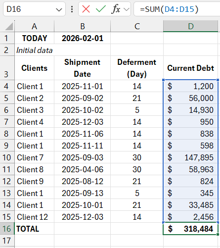
Start sorting debtor companies by creating a company catalog in Excel as shown below:

Using the shipment date information, you can calculate the payment deadline based on the provided grace period. You need to add the number of grace period days to the date when the product was physically delivered.

To add days to the shipment date in Excel, follow this procedure:

Calculating Overdue Days

First, activate the corresponding cell and input the necessary data (without spaces), then activate the fields as follows:

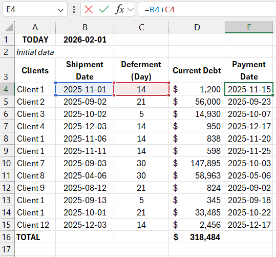
=DATE + NUMBER, then press ENTER.

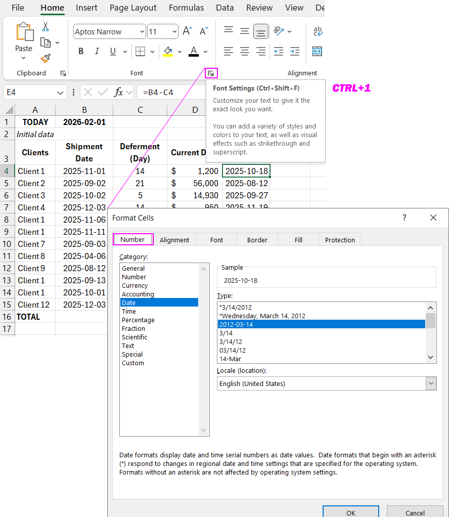
If the date is not displayed correctly in the table, check the field format and ensure it is set to "Date":

If everything is done correctly, the result will look like this:

Now, calculate the overdue days by subtracting the last payment due date from the current calculation date.

To quickly subtract one date from another in Excel, follow this:

Activate the necessary cell and input the required number (without spaces), or activate the cells as follows:

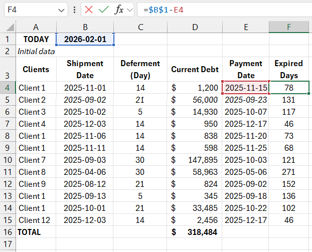
=DATE(1) - DATE(2), then press ENTER.

If the date is displayed incorrectly, check the format. If it is set to something other than "Number," change it.

In this case, use absolute references as we will reference the same date.

Dragging the formula down the Excel table gives the following result:

Now proceed to calculate the penalty interest for the overdue payments.

Calculating Late Payment Penalty

We will consider two possible scenarios:

1. A daily interest of 0.1% was applied to the overdue balance.
2. The refinancing rate at the time of calculation is ten percent.

Penalty Interest Calculation in Excel:

1. Daily interest rate of 0.1%:

Activate the necessary cell in the table and input the values (without spaces) as follows:

=0.1% × overdue balance × number of overdue days, then press ENTER.

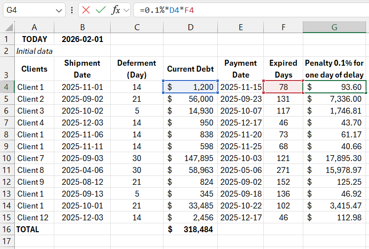
2. Refinancing rate (10%):

Activate the necessary Excel cell, and activate the required fields as follows:

=10% × Debtor's balance/365 × Number of overdue days, then press ENTER.

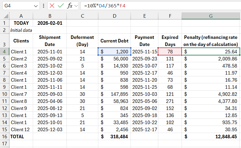
Sum the calculated penalty and the total overdue receivable amount.

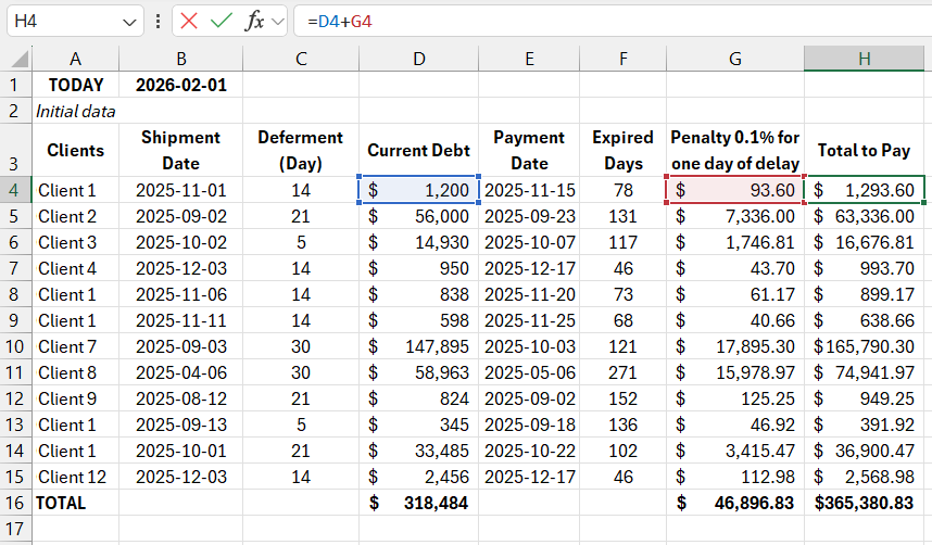
Now rank the debtor companies based on whether it makes economic sense to pursue legal action.

Logical Operator "SUMIF"

Suppose the legal costs amount to 950 rubles per client. To calculate the amount recoverable after winning a case, use the logical operator.

Activate the cell where the total should be calculated. From the menu (highlighted in red), select "Math & Trig," then choose "SUMIF."

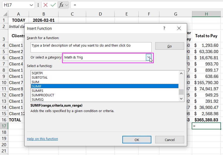
Now let's see what needs to be entered:

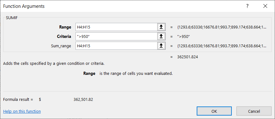
Let’s break it down step by step:

The "Range" box allows you to select the range of values to filter. In this case, it should be the entire last column, excluding the total amount.

The "Criteria" box is used to set the conditions. In this case, the range will be ">950."

The "Sum range" specifies the values to be summed based on the condition. Here, the "Range" and "Sum range" will coincide since the value is directly related to the last column.

After filling in all the fields:

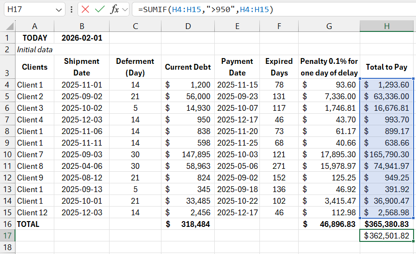
The result shows the total amount that can be recovered after excluding debtors whose total debt is less than 950 rubles (the litigation cost).

For a practical demonstration of SUMIF's capabilities, let’s do another selection of debtors.

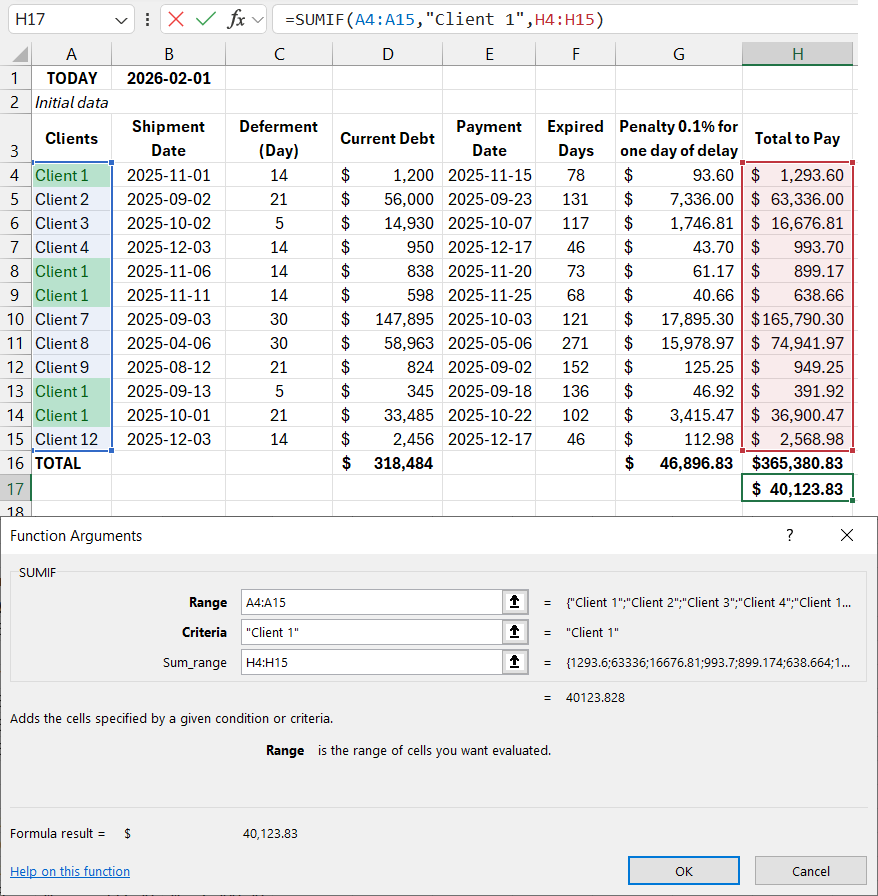
In the previous example, "Sum range" and "Range" were identical. Now, let’s consider a case where different values are specified in these columns.

For example, we need to calculate the debt amount only for "Debtor #1."

In this case, set the "Range" to the first column and manually input "Debtor #1" in the "Criteria" box. Alternatively, select any cell containing this value.

In the "Sum range" box, select the last column, as we need to select the receivable for Debtor #1 from the total amount.

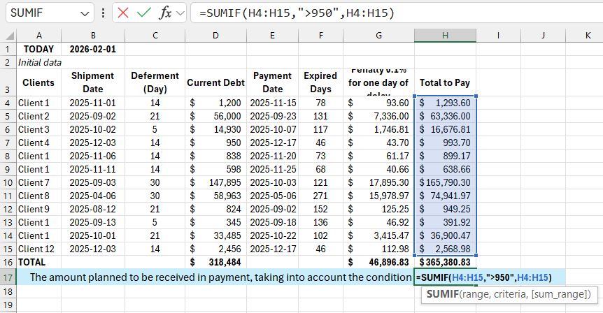
The result will be:

Download Example of SUMIF Formula in Excel for Accounts Receivable Analysis

As demonstrated, the "SUMIF" function in Excel offers a wide range of possibilities and, when used correctly, can provide invaluable assistance in solving many tasks.