Example of Using a Formula in Excel Conditional Formatting
One of the most basic rules for conditional formatting is highlighting cells that meet specific conditions.
How to Set Up Conditional Formatting with a Formula in Excel
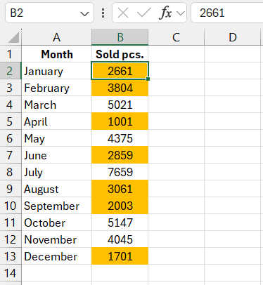
The image below shows a simple sales report. In this example, conditional formatting is applied to dynamically highlight cells with values less than a specified number, <4000:

To create a simple formatting rule, follow these steps:
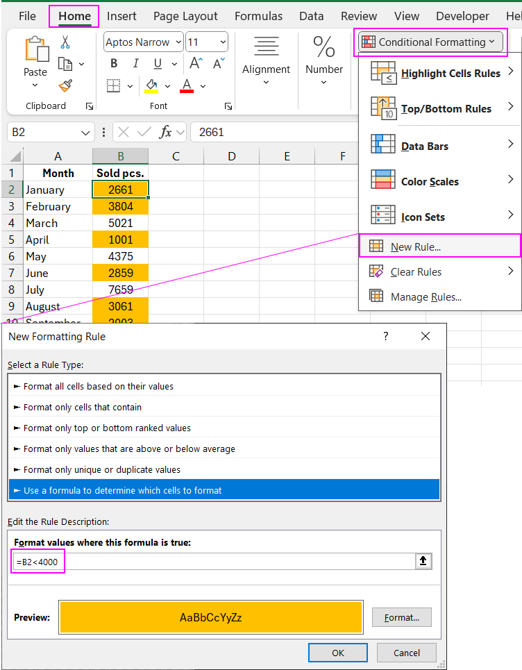
- Select the required range of cells (in this case, B2:B13) and choose: "HOME" - "Conditional Formatting" - "Create Rule." The "New Formatting Rule" dialog box will appear:
- In the list of options at the top of the window, select "Use a formula to determine which cells to format." This option allows you to use a formula to apply formatting. If the formula evaluates to TRUE for any cell, conditional formatting will be applied to that cell.
- In the formula input box, enter the following logical expression. There is no need to specify a reference for the entire range:
=B2<4000
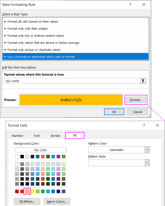
Note that this formula does not include the dollar sign ($) in the reference to the target cell (B2). If you enter the reference by clicking on cell B2, Excel will automatically create an absolute reference. It's essential to avoid using a dollar sign in the relative reference to allow the formatting rule to apply individually to each cell in the range. - Click the "Format" button. The "Format Cells" dialog box will appear, where you can select font, border, and fill options. After choosing the desired formatting options, click "OK" to confirm the changes and return to the "New Formatting Rule" window. Then click "OK" again to apply the conditional formatting to the selected range, B2:B13.


As a result, all cells with values <4000 will be automatically formatted according to the condition.
Editing Conditional Formatting Rules in Excel
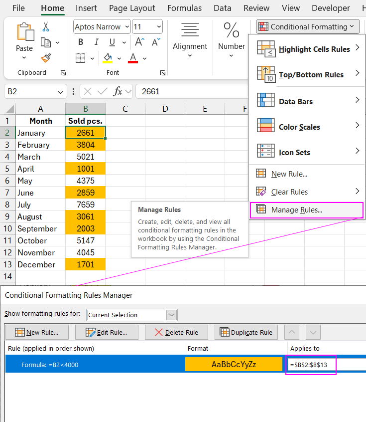
To edit a conditional formatting rule, simply select any cell that is subject to the dynamic format rule, then choose: "HOME" - "Conditional Formatting" - "Manage Rules." The "Conditional Formatting Rules Manager" dialog box will appear. Select the rule you want to edit, then click the "Edit Rule" button.

Download example of using formula for conditional formatting in Excel 
Conditional formatting in Excel refers to the dynamic alteration of cell or range formatting based on specific conditions. This feature allows you to quickly and visually analyze reports and instantly identify key and outlier values.
This article provides several examples of how to use Excel formulas for conditional formatting, which enhance the visual quality of data analysis results. This frequently used and powerful tool in Excel offers extensive functionality.
