Examples of formulas on how to use COLUMN function in Excel

The COLUMN function in Excel returns the column number of a cell on a sheet based on the provided conditions. The syntax is simple: it has only one argument. However, it can be effectively used to solve a variety of tasks.



Description and Syntax of the Function

Function with a parameter: =COLUMN(C3) returns the value 3, as (C) is the third column.

The "reference" argument is optional. It can be a cell or a range from which you need to get the column number.

Argument – reference to a cell:

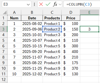
The function returned the column number for this cell.

Argument omitted:

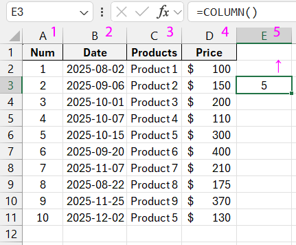
The function returned the column number where it is located.

Argument – vertical range of cells:

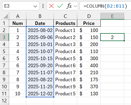
The function returned the column number where the range is located.

Argument – horizontal range of cells:

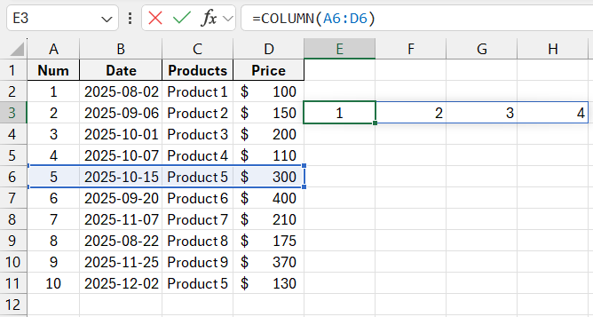
The COLUMN function returned the number of the leftmost column (A) in the specified range. If you highlight the formula in the formula bar and press F9, the program will display all the column numbers of the specified range.

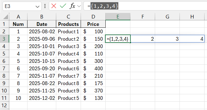
However, when pressing Enter, only the leftmost column number will appear in the cell with the formula.

To display the column numbers of all the columns in the range, you need to use an array formula. Select as many cells as there are elements in the horizontal range. Enter the formula and press Ctrl + Shift + Enter.

Argument – reference to a horizontal array:

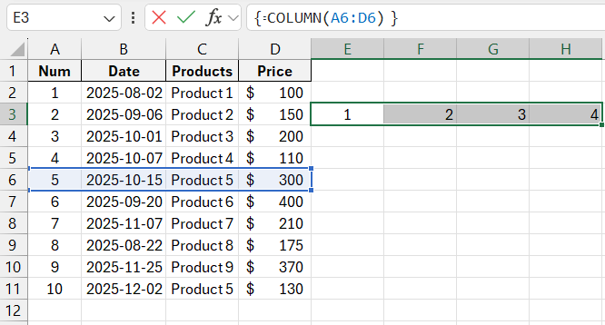
The formula returned the column numbers as a horizontal array.

Note that the argument cannot be a reference to multiple areas.

Useful Examples of the COLUMN Function in Excel

Formulas with the COLUMN function can output a sequence of numbers, which can be applied to solve other tasks.

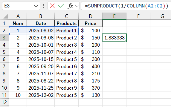
For example, let’s calculate the value of the expression 1 + ½ + 1/3. Use the formula: =SUMPRODUCT(1/COLUMN(A2:C2)).

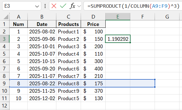
We can perform more complex manipulations with a number series: let's find the sum of values from 1 to 1/n³, where n = 6. The calculation formula is: =SUMPRODUCT(1/COLUMN(A9:F9)^3).

Most often, this function is used in conjunction with the VLOOKUP function. The goal of the first function is to specify the column number of the values to be returned. This combination is convenient when working with large tables. For example, the user can place the returned data in a table with the same column order as the source table, even when both tables are quite wide.

To recap, VLOOKUP searches for a specified value in the leftmost column of a range and returns a value from another column in the same row. Technically speaking, VLOOKUP finds a unique identifier in a database and retrieves related information.

The arguments of the VLOOKUP function: lookup value, data range, column index number, and whether an exact or approximate match is required. You can set the column index number using this formula:

=VLOOKUP(8,$A$1:$D$11,COLUMN(D1),TRUE)

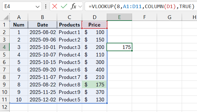
When working with wide tables, you can simply copy the VLOOKUP function horizontally. In this case, the column numbers will automatically recalculate—filling the table accordingly.

If you need to adjust the column index—add or subtract a specific number or a value calculated by another function. For example:

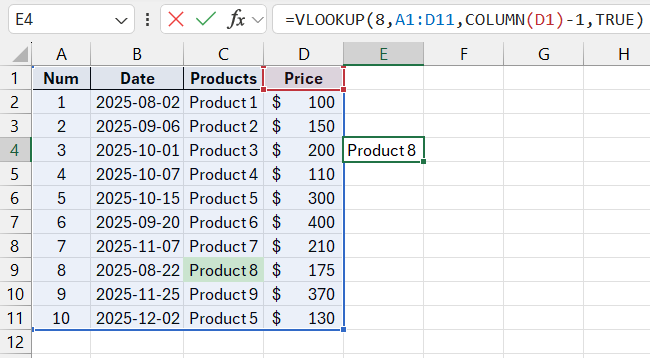
The COLUMN function needs to subtract 1 from the column number of column C. Therefore, VLOOKUP returns a value from the second column of row 9 instead of the third.

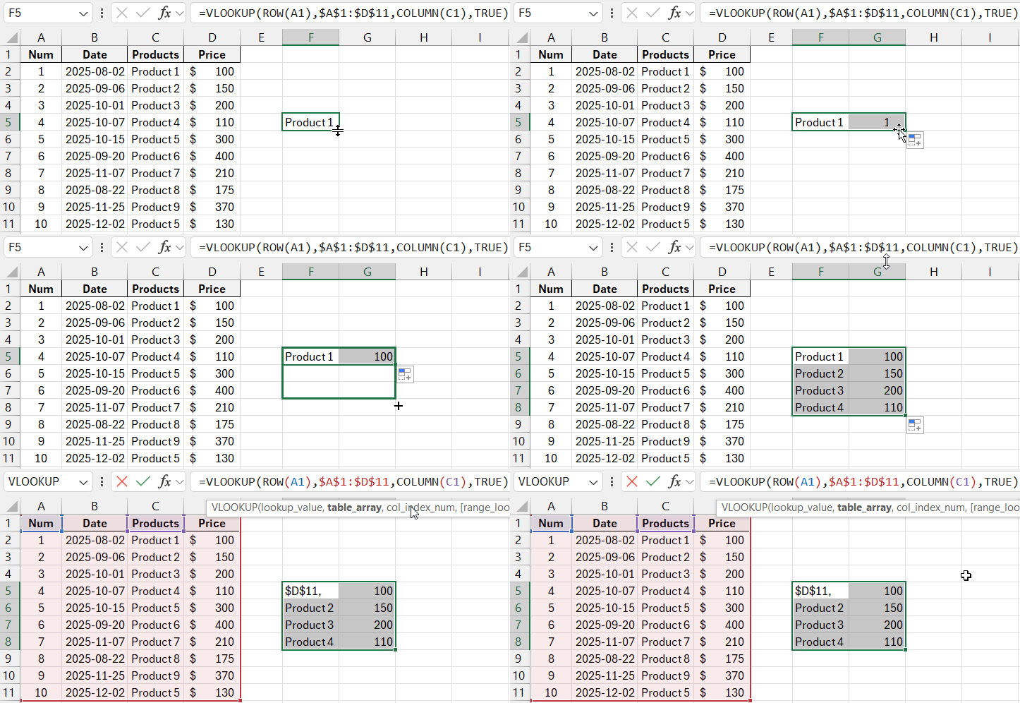
Now let’s illustrate how copying works without the need for manual adjustment. First, lock the references to the table (use the F4 key). Then, copy the VLOOKUP formula across columns—the column number will automatically change (the COLUMN function shifts along with the other references). We will also add the ROW function to the formula.

=VLOOKUP(ROW(A1),$A$1:$D$11,COLUMN(C1),TRUE)

Download example of formula on how to use COLUMN function in Excel

This is an elegant solution that allows you to automatically adjust formulas.