Examples of using SUBSTITUTE function in Excel formulas

Oftentimes when working in Excel, there is a need to dynamically replace one text with another. To address such tasks, the SUBSTITUTE function was created.



Correcting errors in the text using the SUBSTITUTE function

One example of the use of the SUBSTITUTE function is the presence of an apostrophe before the suffix 'S in English company names, which distort the operation of the PROPER function. This function should only change the first letters in words to large, capital ones. And as a result, in the source word where there is an apostrophe, the function returns 2 capital letters, which distorts the result of its work:

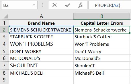
The fact is that the text function PROPER works on the principle of replacing all the first characters with a capital letter that are located after characters that do not correspond to letters: !,?,-,',*,/, etc. Therefore, if there are characters inside a word that are not letters, the operation of the PROPER function will be distorted.

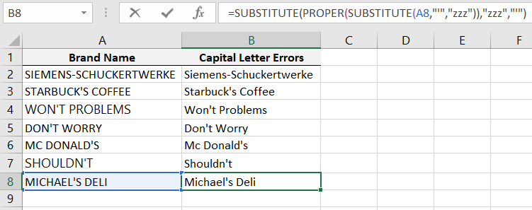
However, by using a simple formula in combination with the SUBSTITUTE function, this drawback can be easily overcome. The example below illustrates the solution to this problem and visually demonstrates the formula in action:

At the core of the above formula is the SUBSTITUTE function, which requires filling in 3 out of 4 mandatory arguments:

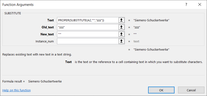
1. Text – the original text or a reference to a cell with the original text in which replacement of characters should be performed.
2. Old_text – the old text to be replaced.
3. New_text – the new text to replace the old one.
4. Occurrence_number – an optional argument. If the string contains several identical old texts to be replaced, this argument can specify which one to replace in order. If this argument is omitted, then all found identical old texts in the original string will be replaced.

If you carefully examine the entire formula, you'll notice that the SUBSTITUTE function is used twice. Not only in the core but also as an argument for the PROPER function. Therefore, to analyze this formula in detail and not get confused, let's break it down into 3 parts since 3 functions are applied.

Part 1:

SUBSTITUTE(A2,"'","zzz")

First, the SUBSTITUTE function is used to replace the apostrophe with the temporary text "zzz." At first glance, this approach may seem unprofessional and meaningless, but it's not. To get the correct result when using the SUBSTITUTE function and at the same time not removing non-letter characters from the text, we have to go for a small trick in Excel. By preserving all characters in the original text. The first part of the formula for the second part will return the following result for further processing:

MICHAELzzzS DELI

Part 2:

PROPER(SUBSTITUTE(A2,"'","zzz"))

The second part of the formula encompasses the first part and works with what the first formula returned to it, namely the same original string but with the temporary text "zzz" instead of the apostrophe "'. Then the affected PROPER function comes into play, which capitalizes the first letters in all words. As a result, we get a textual string like:

Michaelzzzs Deli

Part 3:

=SUBSTITUTE(PROPER(SUBSTITUTE(A2,"'","zzz")),"zzz","'")

Useful tip! Instead of entering the single quote apostrophe character (') in the formula, the function CHAR(39) would be more readable. This function returns the same character by the Unicode table code, as indicated by the code 39 in the CHAR function argument. That is, the following more readable formula returns the same result:

=SUBSTITUTE(PROPER(SUBSTITUTE(A8,CHAR(39),"zzz")),"zzz",CHAR(39))

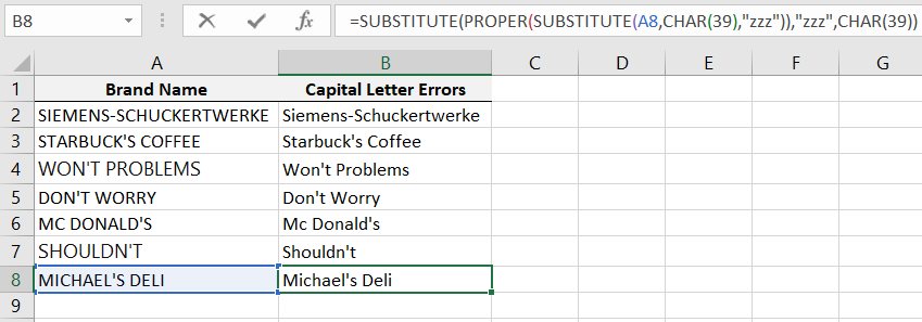
And then it remains to use the SUBSTITUTE function again to replace the temporary text "zzz" with the apostrophe "(')". So that the words regain their original appearance with the same characters.

Michael's Deli

Sometimes, you have to find your own alternative solutions in Excel if there are no standard tools provided.

Other examples of effective use of formulas with the SUBSTITUTE function

Example 1:

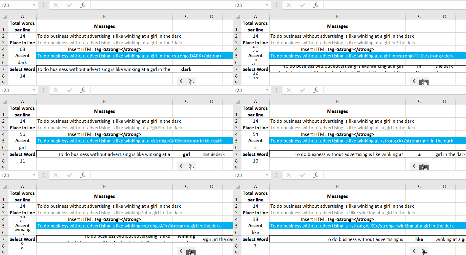
How to Substitute Text for Excel Replacement Formulas

Example 2:

Text functions in Excel formulas: UPPER, LOWER and PROPNOUN

Practical application of the SUBSTITUTE function in Excel

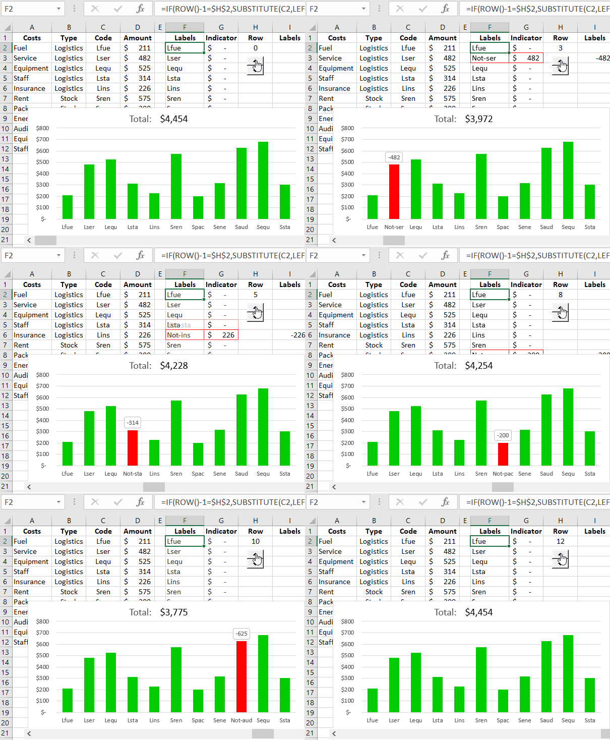
The original data table contains expense articles for transport logistics and warehouse logistics. The corresponding expense amounts for each article are also indicated. It is necessary to create a simple but visual report for analyzing the impact of completely excluding an expense article on the overall expense total for all articles.

For this, using the SUBSTITUTE function, we will exclude the selected expense article from the total list by replacing its name.

First, we will create a table that will transform the original data into the desired format. Next to it, we will make a column for visualization data with dynamic formulas and the SUBSTITUTE function:

=IF(ROW()-1=$H$2,SUBSTITUTE(C2,LEFT(C2,1),"Not-"),C2)

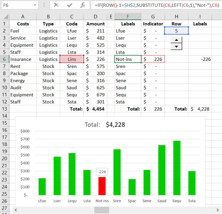
Now, by changing the number of the selected row in cell H2, one of the expense articles is excluded from the total amount:

Download

The user of the visual report has the ability to choose any article for exclusion and, based on the data visualization, make strategic decisions.