Finding Nearest Value in Array and Duplicates in Excel
In this Excel example, we will search for cells with the values closest to a number chosen by the user (whether smaller, larger, or equal—it doesn’t matter, as long as they are as close as possible to the target value).
How to Find the Nearest Higher Value Using a Formula in Excel
Let's start with a simple table that contains a list of names and their corresponding scores.
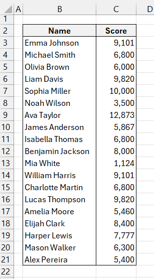
It is worth noting that for some names, the number of points repeats.
We want Excel to return the scores closest to the number entered in the G2 cell of the worksheet, along with the names associated with those values.
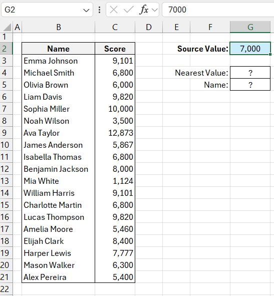
We need to get the closest score and the corresponding name with one query.
Finding the Nearest Value Without Using an Array in Excel
One simple way to solve this problem is to use a helper column. In this column’s cells, there will be the absolute differences between the target number and the scores from the list.
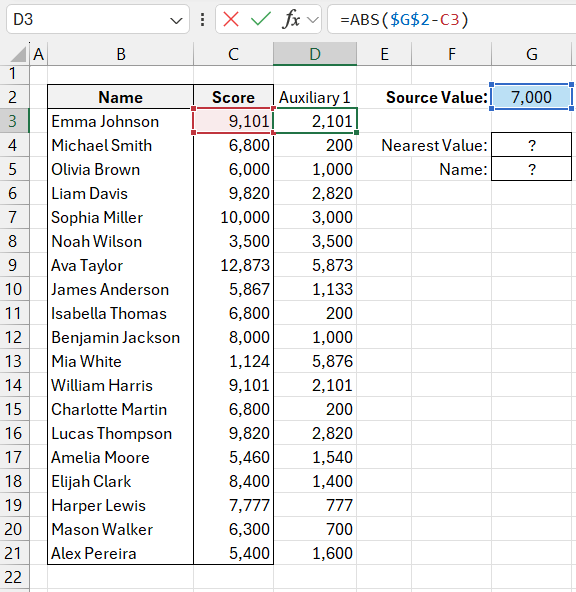
Obviously, the solution to our problem will be found in the row where this difference is the smallest.
To select the corresponding value and its associated name, you can use the following formulas with the INDEX and MATCH functions. For the nearest value:
=INDEX(C3:C21,MATCH(MIN(D3:D21),D3:D21,0))
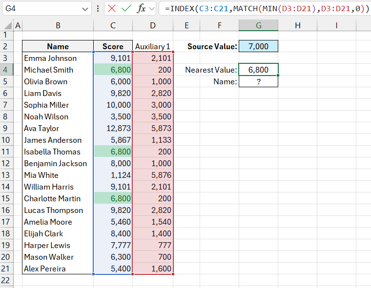
For the name corresponding to the nearest value:
=INDEX(B3:B21,MATCH(MIN(D3:D21),D3:D21,0))
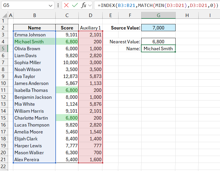
Here, column “D” is our helper column, and column “B” is the column with the names. Just to clarify, column “C” contains the score values.
Finding the Nearest Value in an Excel Array
A “hardcore” solution using array formulas (for enthusiasts or those who just want to practice creating array formulas).
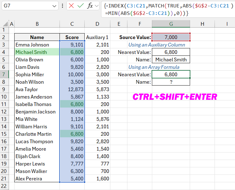
Finding the nearest value in an array (CTRL+SHIFT+ENTER):
=INDEX(C3:C21,MATCH(TRUE,ABS($G$2-C3:C21)=MIN(ABS($G$2-C3:C21)),0))
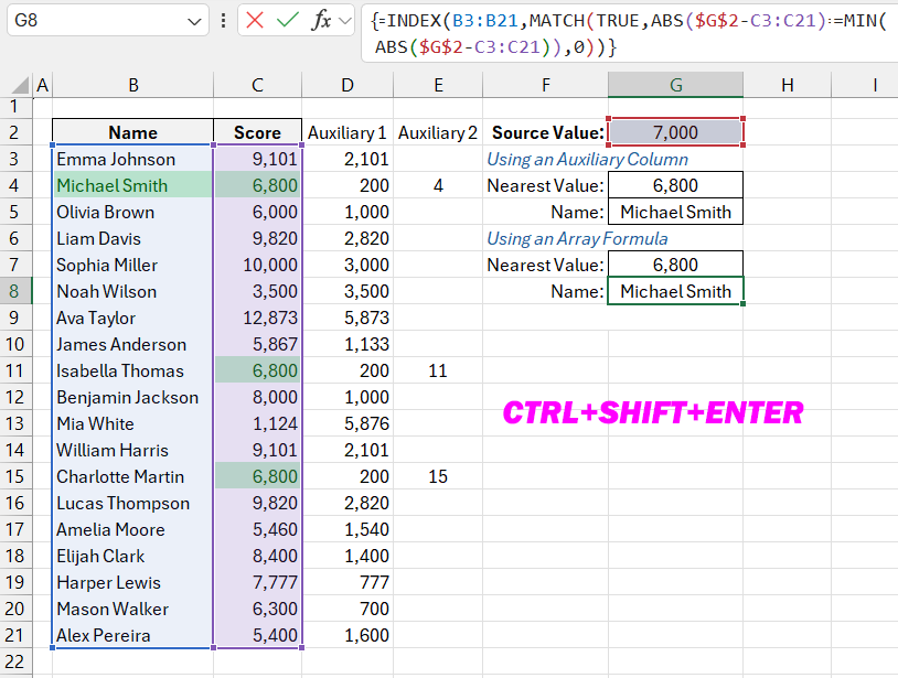
Finding the corresponding name in an array (CTRL+SHIFT+ENTER):
=INDEX(B3:B21,MATCH(TRUE,ABS($G$2-C3:C21)=MIN(ABS($G$2-C3:C21)),0))
Duplicate Nearest Values in Excel
The two methods shown above return only one value. So, when multiple names correspond to equal scores, the formula will return only the first name in the list.
So, how can you make Excel return a list of all the names with the scores that meet the desired criteria when there are duplicates of the nearest values?
There are two solutions using a helper column. The first without, and the second with the use of array formulas.
First, prepare the helper column. The first cell will contain the following formula:
=IF(ABS($G$2-C3)=MIN($D$3:$D$21),ROW(),"")
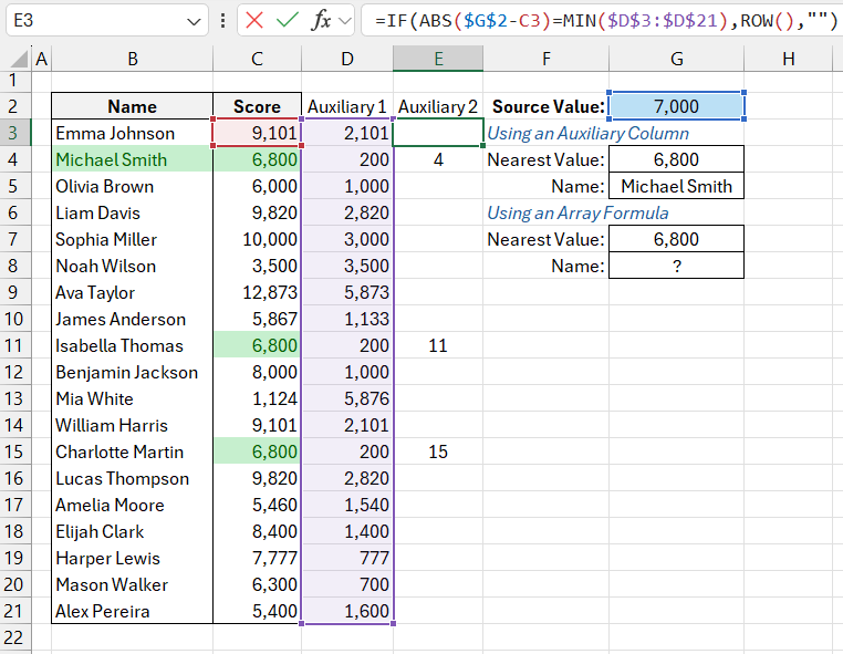
which you then drag (copy) into the other cells of the helper column.
The formula should return the row number where the value is closest to the target. Otherwise, it returns a blank space.
Without Using Array Formulas
The helper column is now ready, and we can return to our search.
In the first cell of the range where you want to have a list of all names, enter the following formula:
=INDEX(B:B,SMALL($E$3:$E$21,COUNTA($F$10:F10)))
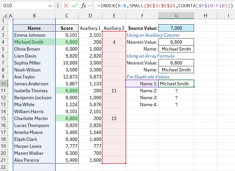
And in the cell below, which will return the next name, enter the formula:
=INDEX(B:B,SMALL($E$3:$E$21,ROW($A$1:INDEX($A:$A,COUNTIF(E3:E21,">0")))))
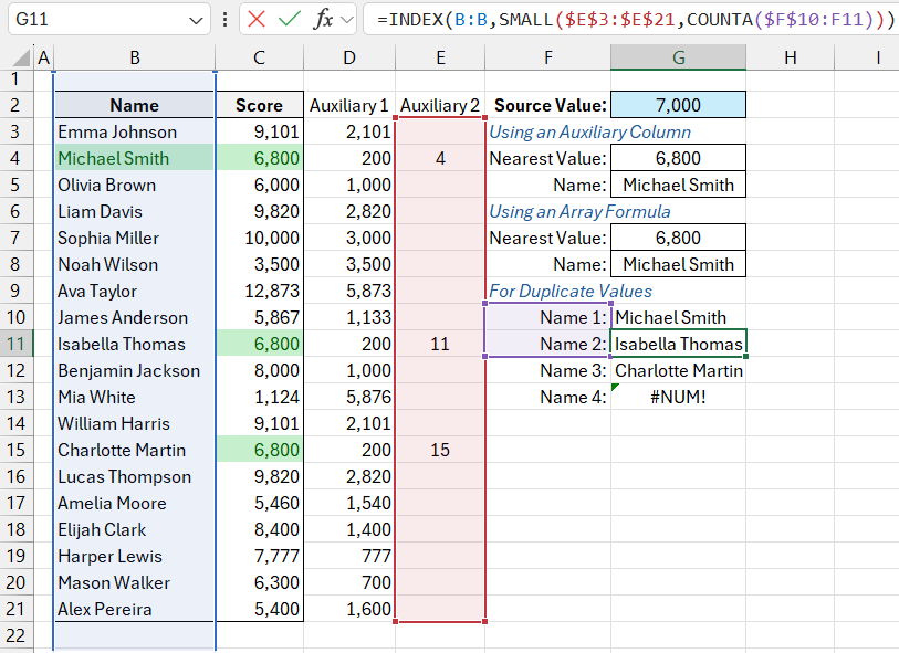
which you can then copy further down. The result should look something like what is shown in the image below. As you can see, these formulas give you a list of all the names that meet the search criteria.
Finding Duplicate Nearest Values in an Excel Array
Finally, the same task but using array formulas (we will use the helper column described earlier).
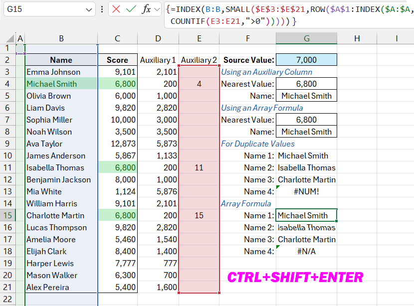
Select the range of cells where you want the list of names (e.g., G15:G19) and use the array formula:
=INDEX(B:B,SMALL($E$3:$E$21,ROW($A$1:INDEX($A:$A,COUNTIF(E3:E21,">0")))))
Download an Example of Finding the Nearest Value in Excel 
The formula will return exactly what you expect. In all the cells that do not match the criteria, the formula will return an error code. If necessary, these can be easily removed or wrapped in the IFERROR function.
