Formula for Automatic Formatting Based on Value in Excel
It often happens that a formatting rule for a cell must take into account the values of other cells. This is very convenient, as it allows users to dynamically change the format of cells by adjusting the value in one cell. Let’s explore this situation with an example and its solution.
How to Automatically Change Formatting Based on Cell Value in Excel
The image below shows a table where cells are conditionally formatted based on whether their values are less than the number in the "Average" cell at address A2.
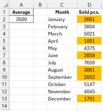
To create such a simple dynamically formatted condition, follow these steps:
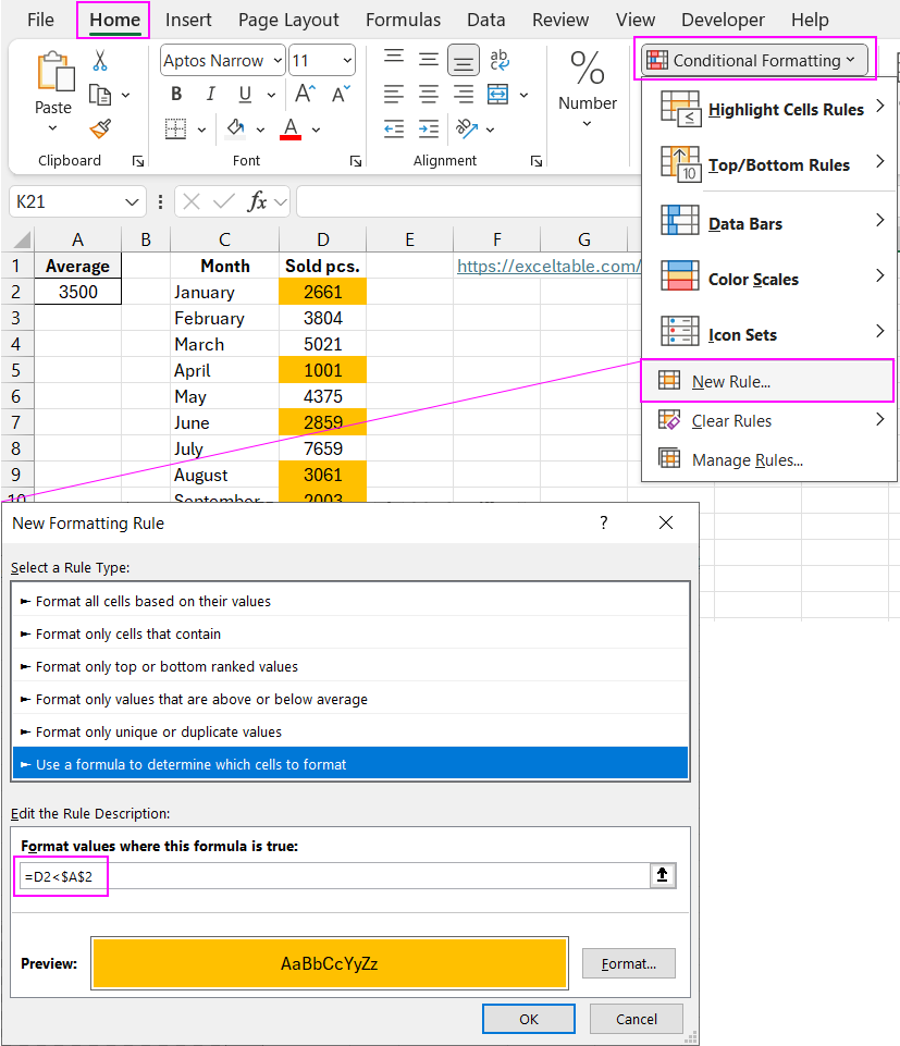
- Select the target range of cells (in this example, $D$2:$D$13) and choose: "HOME" - "Conditional Formatting" - "Create Rule." The "New Formatting Rule" dialog box will appear, as shown below:
- From the list at the top of the window, select the option "Use a formula to determine which cells to format." This option allows you to apply formats based on a specific formula. If the formula returns TRUE for any of the cells, conditional formatting will be applied to that cell.
- In the formula input field, enter the logical expression shown at this step. This formula simply compares the value of the target cell D2 with the value in the reference cell at address $A$2. Just as with standard formulas, you need to make sure that the reference to the comparison cell is absolute so that the value of each cell in the selected range is compared with the value in $A$2:
=D2<$A$2
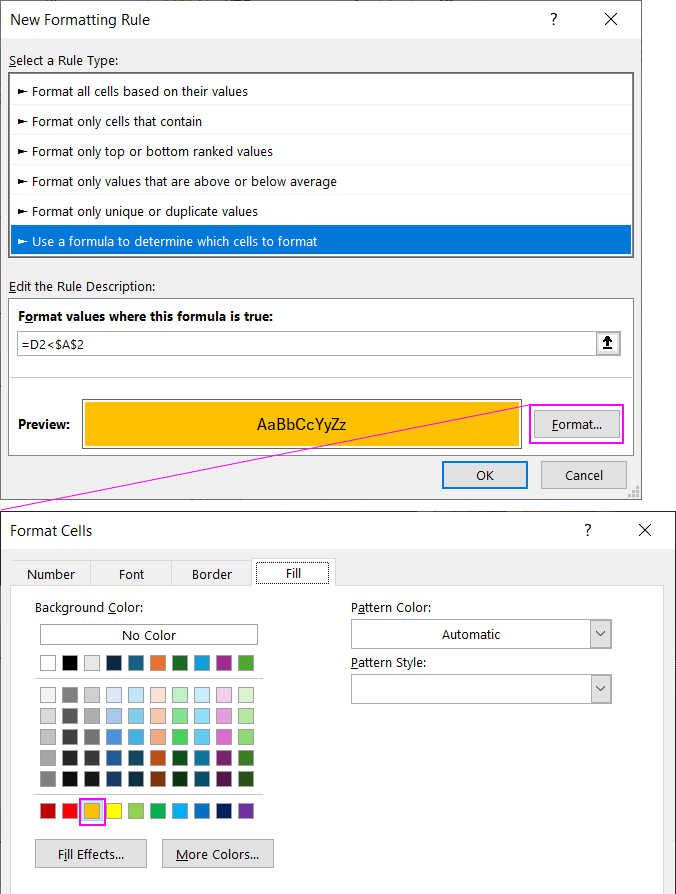
Notice that there are no dollar signs ($) in the reference to the first target cell D2 in the above formula. If you don't enter the address manually and click on cell D2, Excel will automatically create an absolute reference =$D$2. It's important that there are no dollar signs in the references to the target cells so that the formatting rule can be applied separately to each cell in the range $D$2:$D$13. - Click the "Format" button, and the "Format Cells" dialog box will appear, where you can choose formatting options for fonts, borders, and fills. After specifying the necessary formatting options, confirm them by clicking "OK" in all open windows.
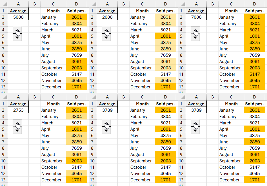
As a result, we get a dynamically changing report based on the condition specified in the formula, which the user can modify by changing the value in cell $A$2:

Download formula example for automatic formatting based on value in Excel 
As soon as the value is changed, different cells are automatically highlighted.
