Formula for Calculating Months Passed Since Date in Excel
Sometimes in Excel, it's necessary to calculate the number of years and months between two dates. For example, between November 23, 1960, and May 13, 2014, 53 years and 5 months have passed.
How to Determine Years and Months Passed Since a Date in Excel?

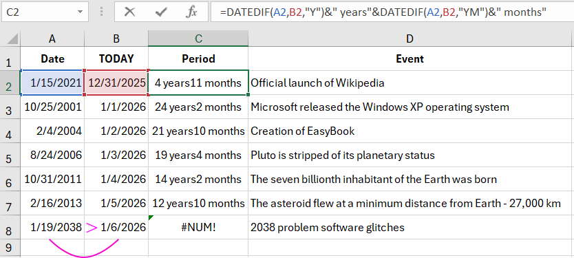
The formula used to determine the elapsed time in years and months between two dates requires the use of 2 functions and a couple of text strings. Cell C2 contains the following formula, as shown in the image:
=DATEDIF(A9;B9;"Y")&" years "&DATEDIF(A9;B9;"YM")&" months"

Note: In cell C9, there is an error: #NUMBER! since the start date is later than the end date, which, by the definition of the DATEDIF function, is incorrect. The value in the first argument of the function must always be less than the value in the second argument.
The necessary calculation is performed using the same DATEDIF function with different values in the third argument. Therefore, the function needs to be called twice. Additionally, for readability, text characters that are joined by the ampersand "&" are added to the formula.
The first DATEDIF function in the formula contains the code "Y" as the time unit and calculates how many years have passed between the two dates: the start and end.
The second DATEDIF function in the formula contains in its third argument the code "YM". Thanks to this, it calculates the number of elapsed months in an incomplete year without considering the full elapsed years between the same two dates.
Finally, both functions in the formula are combined into strings with a textual description so that the user can clearly and easily read which number represents years and which represents months. This is because the result of the formula, two numerical values, is located in one cell.
Applying the Date Difference Calculation Formula
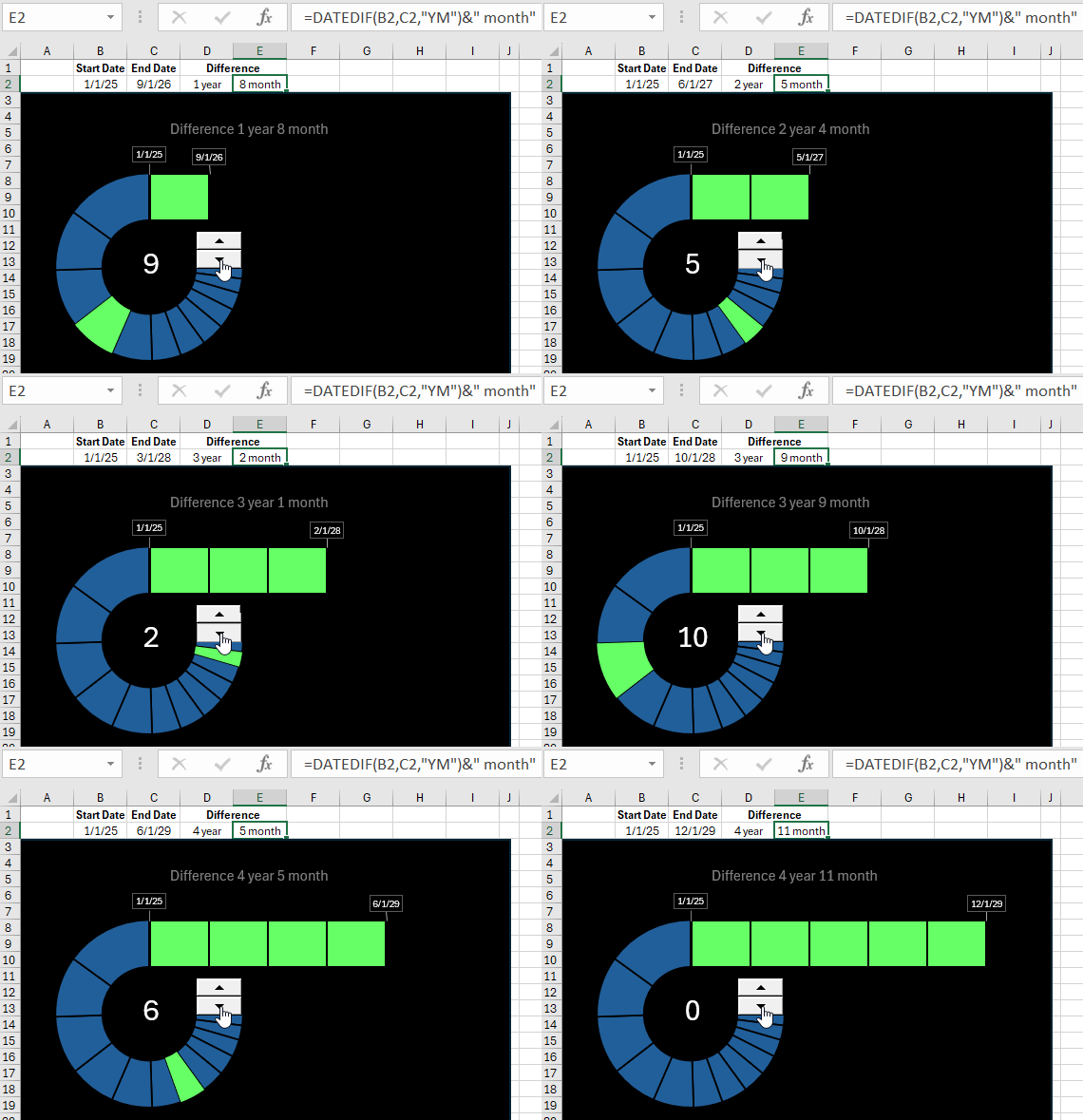
On the dashboard, it is advisable to add a designer element to visualize the difference between two dates in the style of a distance scale.
The design of the element will consist of a combination of a circular diagram and a horizontal histogram. However, label elements will refer to cells with the result of the formula =DATEDIF():

This visualization block has interactive capabilities thanks to the Spinner control element. When used, values in the source cells change, labels are updated, and the magic happens in the data presentation visualization.
 Download