Formula for Extracting Multiple Largest Values in Excel

The MAX and MIN functions are great for finding the highest and lowest values in a data range. However, if you need to find several largest or smallest values, Excel offers additional useful functions: LARGE, SMALL, RANK, and RANK.AVG.



Example of Extracting Multiple Largest Values in Excel

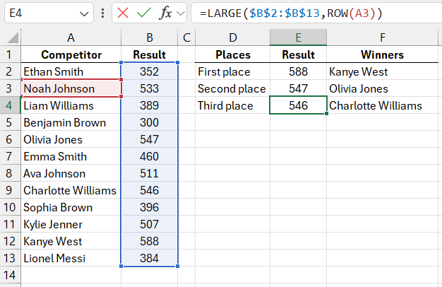
Below is a table showing the results of a bowling tournament. The participants in the leaderboard are sorted alphabetically by name, making it hard to tell who the winner is. Suppose we need to find out which participants ranked in the top 3 and what their scores were. The formula below returns the third-highest score from the list of results:

The formula used to find the participant’s name combines the INDEX and MATCH functions:

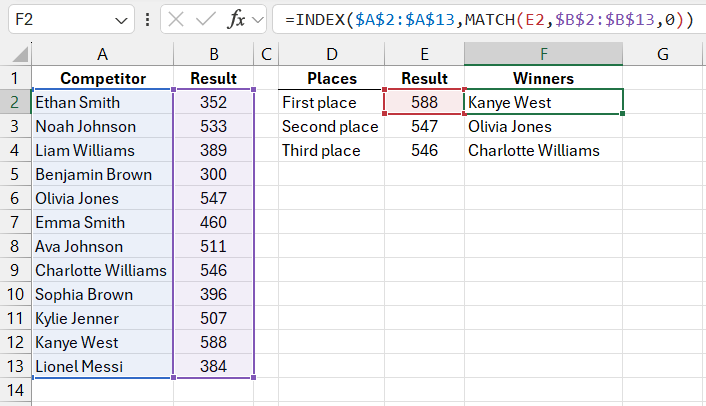
The LARGE and SMALL functions are used to find the nth largest or smallest value in a data list. The first argument in the LARGE function, like in the MAX function, refers to the data range being searched. However, the difference is that the LARGE function has a second required argument, "k", where you specify the rank of the value you want to return (second-largest, third-largest, etc.).

If the data range contains duplicate maximum values, the LARGE and SMALL functions return the same result for consecutive ranked values (k and k+1). For example, if two participants scored 588 points each, the formulas =LARGE($B$2:$B$13,1) and =LARGE($B$2:$B$13,2) would return the same number: 588.

In cell E2, the ROW(A1) function is used to determine the value of the "k" argument. The ROW function returns the row number of the sheet for the cell specified in the argument—here, it’s row 1. Instead of simply typing 1 for the second argument of the LARGE function, the ROW(A1) allows the row number to automatically update when the formula is copied to the cells below. The reference to cell A1 is relative, so when the formula is copied to cell E3, the ROW function will update to ROW(A2). As a result, the LARGE function in cell E3 will return the second-largest value from the "Result" column in the data list.

Ranking Formula in Excel for Extracting Largest Values

In this example, the LARGE function is essential because we’re analyzing bowling scores, where a higher number is better. If we were analyzing another sport where the results were based on time, then the winner would be the one with the lowest time. Below is a leaderboard with time-based results. The table includes an additional column with each participant’s ranking, and the formula used is:

=RANK(B2,$B$2:$B$13,1)

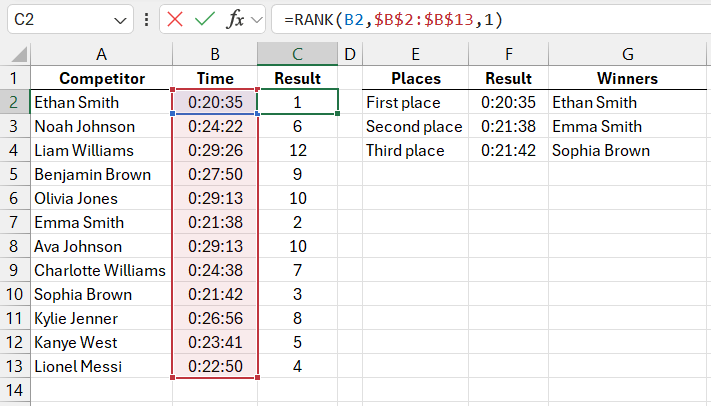
To determine the rank of the participant named "Volchok Gennady," you need to fill in the arguments for the RANK function. The first argument should be the current participant’s time (using a relative reference from cell B2), while the second argument should be an absolute reference to the data range being reviewed, $B$2:$B$13. The third argument determines the order of sorting. In this case, it's 1 because the lowest time should rank first, meaning the order is ascending. If you wanted the highest value in the data range to rank first, you would use 0 for the third argument.

Unlike the LARGE and SMALL functions, the RANK function returns the actual position number for each value. In other words, RANK returns the position of the value in a sorted list based on the last argument. To get the value from a specific cell, you can use a combination of INDEX and MATCH, similar to how participant names were retrieved earlier.

The formula in cell F3 returns the time of the participant who finished third:

=INDEX($B$2:$B$13,MATCH(ROW(A1),$C$2:$C$13,0),1)

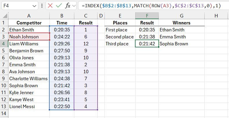
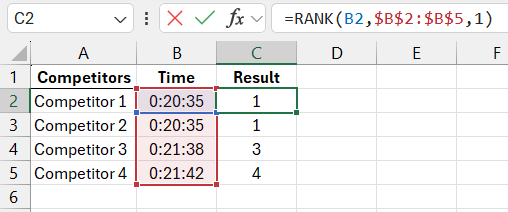
If the data range contains two or more identical values, the RANK function will return the same rank for both. For example, if two participants finished with the same time of 20:35, the RANK function will return 1 for both. The next fastest time will rank third. No value will be ranked second since the two identical values are tied for first:

RANK.AVG Function for Ranking Lists with Duplicates

Starting with Excel 2010, two new ranking functions were introduced: RANK.EQ and RANK.AVG, which handle duplicates differently. The RANK.EQ function behaves similarly to the RANK function, returning the same result for tied values. However, the RANK.AVG function returns the average rank for all identical values.

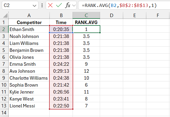
Suppose the table contains results for four participants with the same second-fastest time of 21:38:

Скачать пример использования формулы RANK.AVG в Excel

For the fastest time, the RANK.AVG function naturally returns 1, while for the four participants with the same second-fastest time, it returns an average rank of 3.5. These four participants simultaneously occupy positions 2, 3, 4, and 5, and the ranks are divided equally among them. So, each participant gets a rank of 3.5 (2+3+4+5/4=3.5).