Formula for get Statistical Outliers with Sampling in Excel
In data analysis, it's common to observe that most values cluster around a central point, typically the median. However, some values may deviate significantly from the center. These values are called statistical outliers (falling far outside the expected range). Outliers can distort statistical analysis results, leading to false or misleading conclusions about the data.
How to Identify Statistical Outliers and Sample Them for Removal in Excel
To detect and highlight statistical outliers from the median, you can use several simple formulas combined with conditional formatting.
The first step in identifying statistical outliers is determining the central point of the data range. To do this, we first calculate the boundaries of the first and third quartiles. Quartile boundaries divide the data into four equal groups, each containing 25% of the data. The group containing the top 25% of values is called the first quartile.
Quartile boundaries in Excel can easily be determined using the QUARTILE function. This function requires two arguments: the data range and the quartile number.
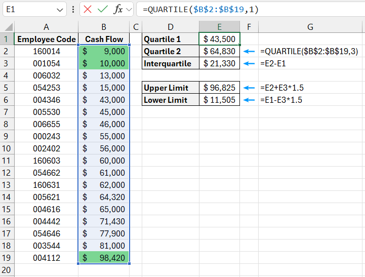
In the example below, the values in cells E1 and E2 represent the first and third quartiles for the data range B2:B19:

By subtracting the first quartile from the third, you can calculate the interquartile range (IQR), representing the middle 50% of the data. The interquartile range is shown in cell E3.
Now the question arises: how much can a value deviate from the middle 50% and still be considered normal? Statisticians agree that the boundaries for determining outliers can be set by multiplying the interquartile range by an expansion factor of 1.5. Thus:
- The lower boundary of the data range is: the first quartile – 1.5 * interquartile range.
- The upper boundary of the data range is: the third quartile + 1.5 * interquartile range.
As shown in the example, cells E5 and E6 contain the calculated upper and lower boundaries of the data range. Any value above the upper boundary or below the lower boundary is considered a statistical outlier.
To visually enhance the data analysis, you can create a simple conditional formatting rule to highlight these outliers.
Sampling Statistical Outliers Using Quartiles in Excel
To create the conditional formatting rule as described above, follow these steps:
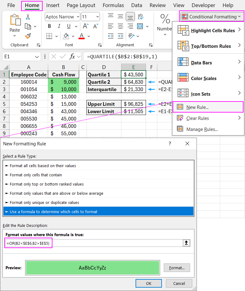
- Select the target cell range (in this example, B2:B19), and navigate to "HOME" – "Conditional Formatting" – "Create Rule." The "New Formatting Rule" window will appear, as shown below:
- In the top section of the window, choose "Use a formula to determine which cells to format." This option is used to analyze the values in the selected range based on a formula with a logical expression. If the formula returns TRUE for any cell, conditional formatting is applied to that cell.
- In the formula input field, enter the logical expression provided here. Note that the formula uses a relative reference for the target cell B2, and absolute references for the upper and lower boundaries in cells $E$5 and $E$6. The two logical expressions are placed inside the OR function. If the value in the target cell is greater than the upper boundary or less than the lower boundary, the formula returns TRUE, and conditional formatting is applied:
=OR(B2<$E$6,B2>$E$5)
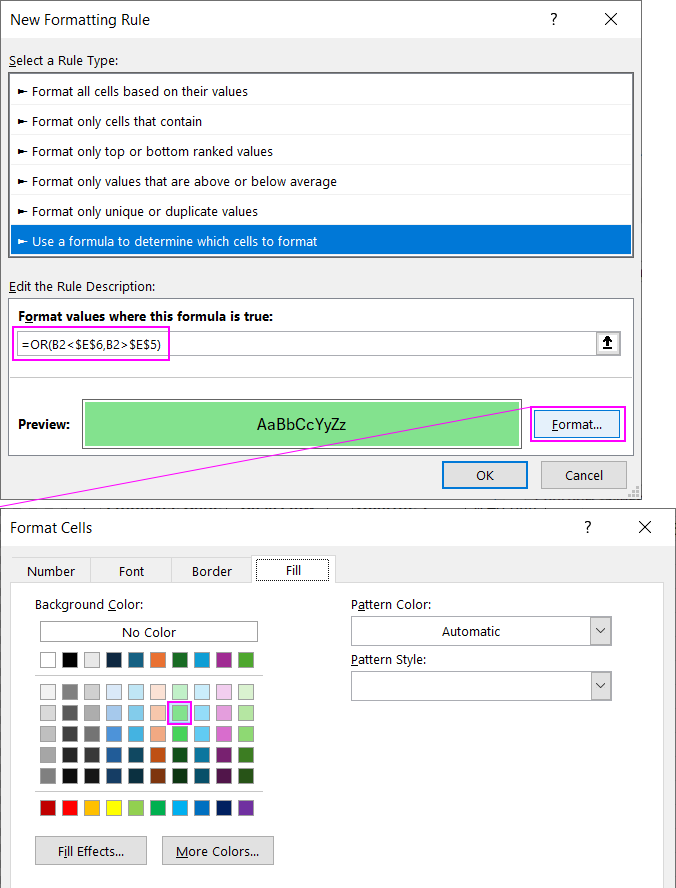
- Click the "Format" button, and the "Format Cells" window will appear, allowing you to set the formatting options for fonts, borders, and cell fill. After specifying the desired formatting, click "OK" on all open windows to apply the rule and complete the process.


Download Example of Formula for get Statistical Outliers with Sampling in Excel 
As a result, all cells containing statistical outliers from the median will be highlighted in color.
