How to Calculate Percentile Using Formula in Excel
A percentile scale determines the position of a specific value among other data in a dataset. Percentiles are primarily used to describe standardized test results. If a result is in the 90th percentile, it means the result is higher than 90% of all other test scores. In other words, it falls within the top 10% of the scores.
Example of Calculating Percentile Formula in Excel
Percentiles (also known as percentiles or percentiles) are frequently used in data analysis to evaluate performance within a group. For example, you can use them to rank employees based on their annual sales performance.
In Excel, you can easily calculate percentile rankings using the PERCENTILE function. This function requires two arguments:
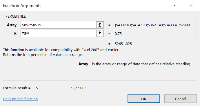
- Array – The range of data values.
- K – The percentile value (usually a decimal between 0 and 1).
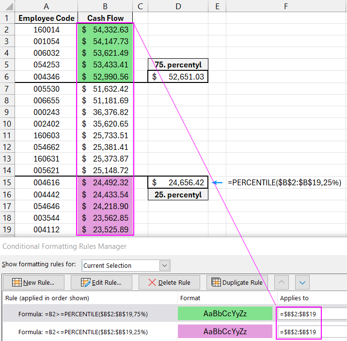
In the example below, the value in cell D6 is the result of calculating the 75th percentile for the data range $B$2:$B$19:
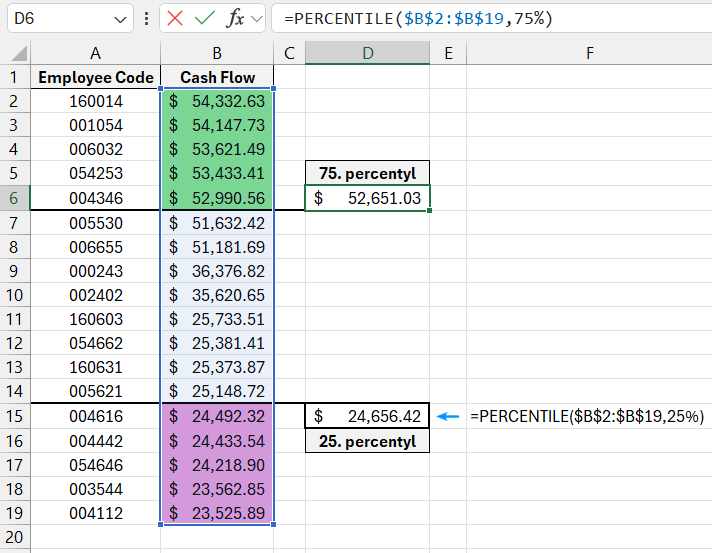
The result of the formula indicates that any employee with annual sales exceeding 52,651 performs better than 75% of all other employees.
Similarly, the value in cell D15 is the result of calculating the 25th percentile for the same data range.
This result shows that employees with annual sales less than or equal to 24,656 are among the bottom 25% of the performers.
In this example, conditional formatting is applied based on the percentile values. Values above the 75th percentile are highlighted in green, while values below the 25th percentile are highlighted in red.
Two Conditional Formatting Rules for One Cell Range in Excel
To create an automated cell highlighting system as described, follow these steps:
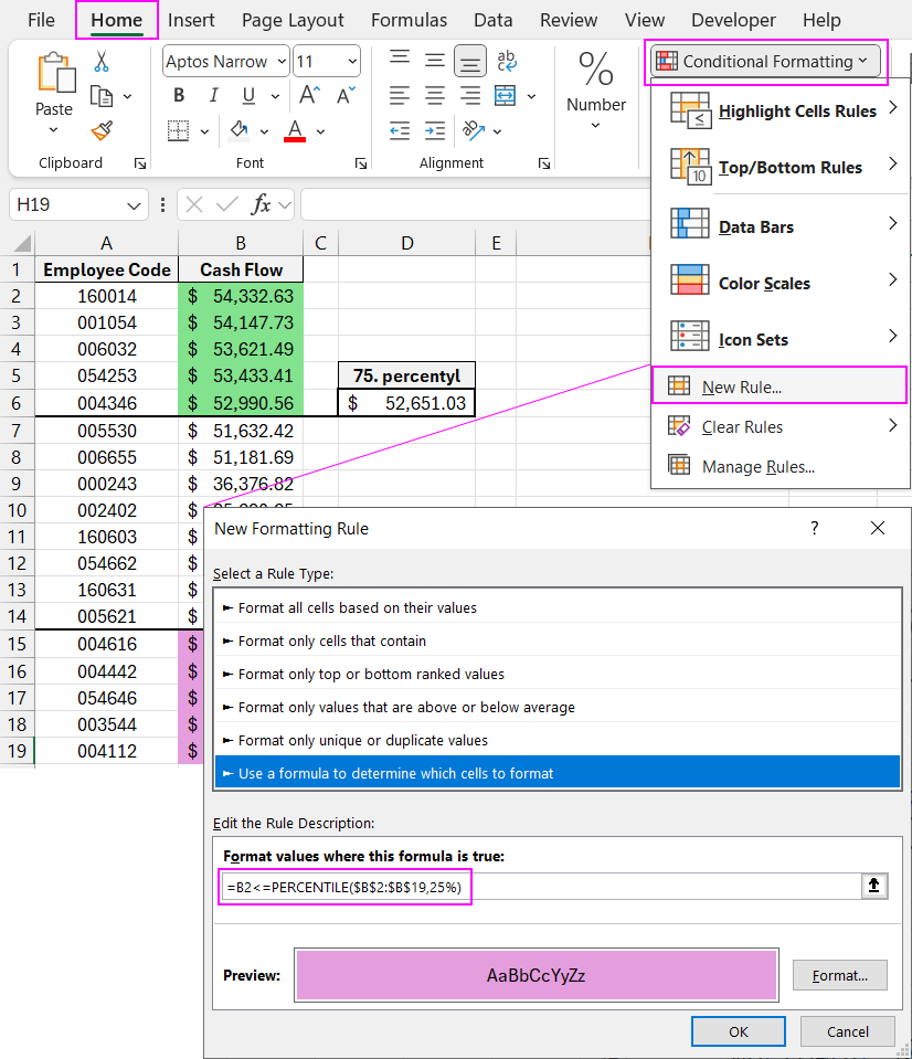
- Select the range of cells (B2:B19) that need to be automatically color-highlighted based on the percentile formula, and go to: "HOME" – "Conditional Formatting" – "Create Rule." A window like the one below will appear:
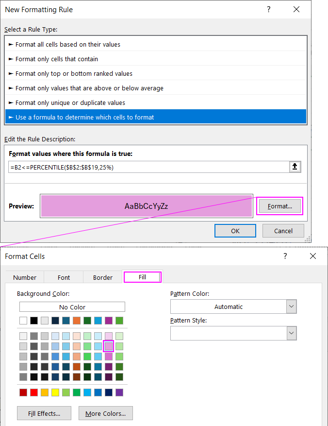
- Select the option "Use a formula to determine which cells to format." This option allows formatting based on a custom formula with logical expressions. If the formula returns TRUE, conditional formatting is applied to the current cell.
- In the formula input field, enter the following formula. This formula checks if the value in cell B2 is less than or equal to the 25th percentile, then assigns a red background:
=B2<=PERCENTILE($B$2:$B$19,0.25)
- Click the "Format" button to open the "Format Cells" window. Here, you can set the formatting options, such as font style, border, and cell fill. Choose a red fill background. After specifying your options, click OK on all open windows to confirm and apply the changes.
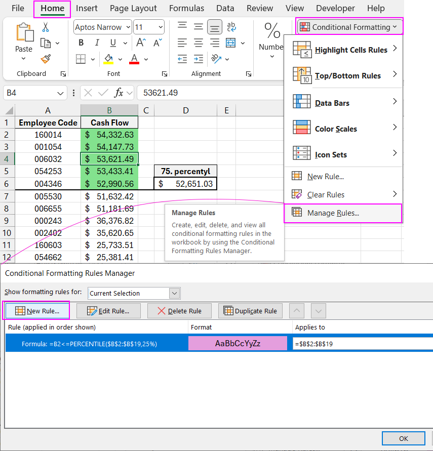
- Select the range B2:B19 again and choose "HOME" – "Conditional Formatting" – "Manage Rules." The "Conditional Formatting Rules Manager" will appear, showing the first rule. To create a second rule, click "New Rule."
- Again, select "Use a formula to determine which cells to format."
- In the formula input field, enter a new formula that checks if the value in B2 is greater than or equal to the 75th percentile. If TRUE, apply a green background:
=B2>=PERCENTILE($B$2:$B$19,0.75)
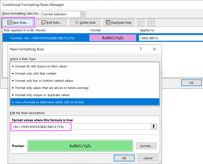
- Click "Format" again and choose a green fill for the cells. Click OK to apply the formatting.
Download Example of Calculating Percentile Using Formula in Excel 
As a result, two conditional formatting rules are applied to the same range of cells. Values in the bottom 25% are highlighted in red, and values in the top 75% are highlighted in green.

Data Visualization Charts for Interactive Report Creation in Excel.
Dashboard Templates