How to Compare Two Lists or Tables Using a Formula in Excel
It is often necessary to compare two lists and select only the values that are present in both lists. Conditional formatting is an excellent tool for such comparisons between two tables in Excel.
How to Compare Two Lists in Excel
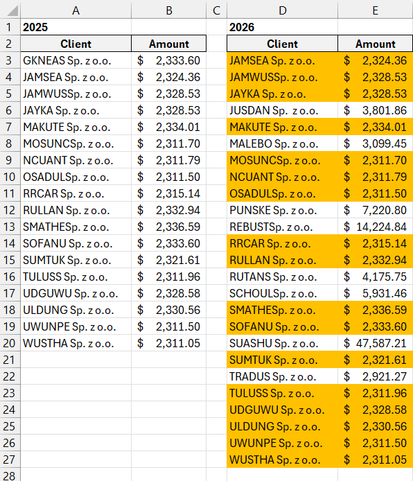
The image below shows an example where customer names are compared across two lists for the period of 2025-2026. Loyal customers appear in both lists:

To create this formatting rule, follow the steps below:
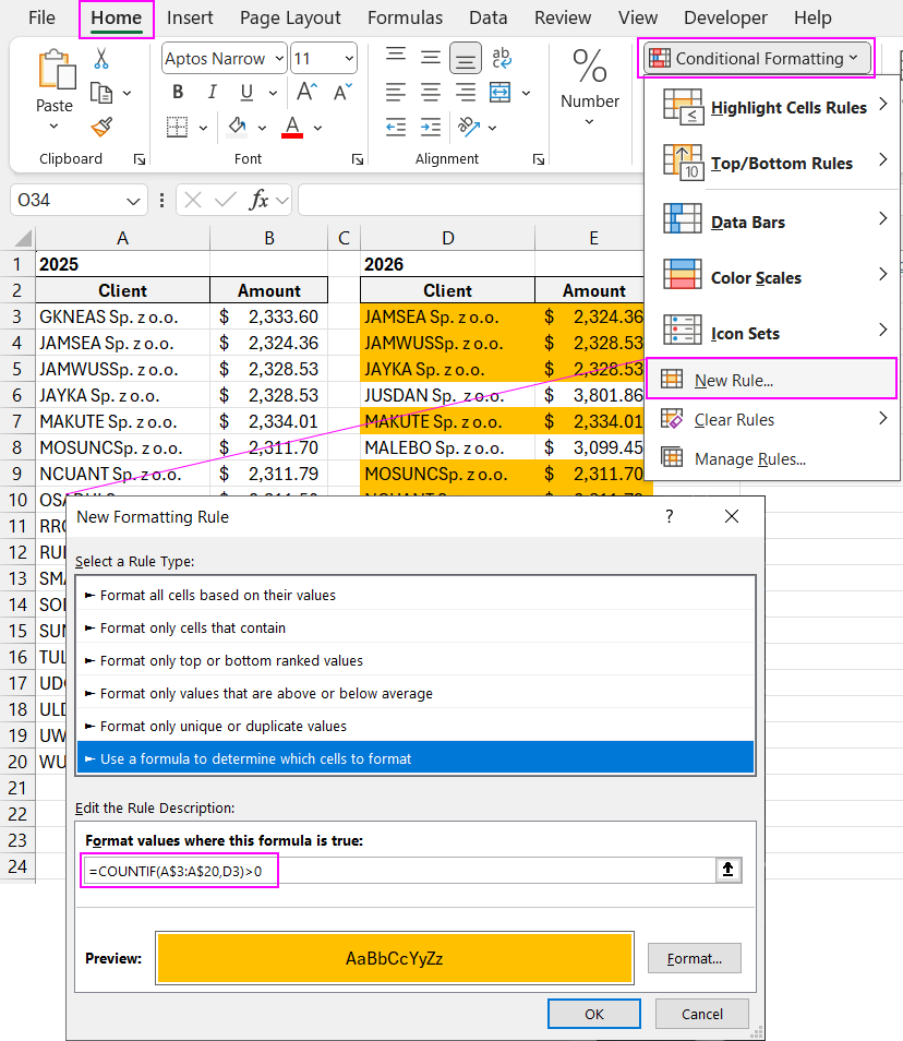
- Select the initial range of cells (in this example, it's A$3:A$20) and navigate to: "HOME" - "Conditional Formatting" - "Create Rule". A window titled "New Formatting Rule" will appear, as shown below:
- From the list at the top of the window, choose the option "Use a formula to determine which cells to format." This feature allows you to apply a formula that reads and evaluates values according to a specific user-defined condition. If the value meets the logical condition of the formula, it will return TRUE, and the new format, pre-set by the user in this tool, will be applied to the respective cell.
- In the formula input field, enter the logical expression as shown in this step. Notice that the check here determines if the value of the target cell D3 is present in the range A$3:A$20. The formula is implemented using the COUNTIF function. If the value is found, the function will return a number greater than 0. In that case, the entire formula will return a TRUE result, triggering the conditional formatting for the current cell. As with standard formulas, ensure that absolute references are used for the range being checked and a relative reference for the target cell. This ensures that each cell in the target range is compared individually against all values in the checked range.
=COUNTIF(A$3:A$20,D3)>0
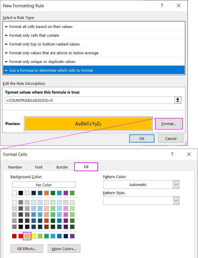
- Click the "Format" button to open the "Format Cells" window, where you can set the formatting style by specifying things like fill color, font size, border thickness, etc. Then click OK in all open windows and enjoy the result.


Download example formula for comparing two lists in Excel 
As a result of comparing the two customer name lists in Excel, only the loyal customers are highlighted.
