How to Convert Date to Quarters in Excel for Fiscal Year
Many of us work in companies where the fiscal year does not start in January but in October, April, or any other month. In such companies, the fiscal year quarters cannot be calculated the same way as traditional calendar year quarters.
Formula for Converting Date to Fiscal Year Quarters
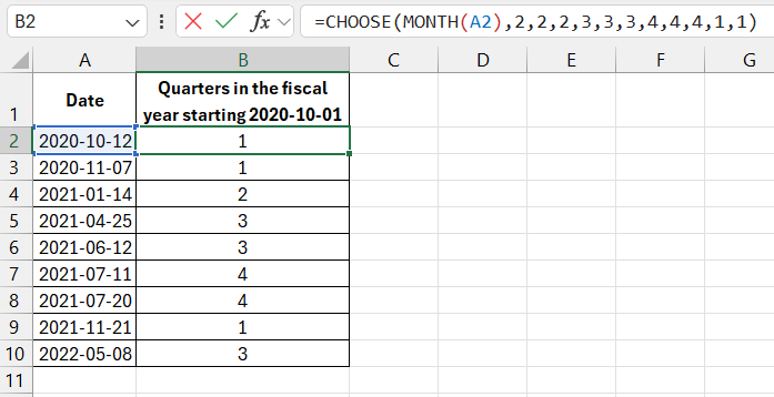
Below is an example formula using the =CHOOSE() function to calculate the quarter for any fiscal period based on specified start dates. In this example, quarters are calculated for a fiscal year starting in October.

The idea behind this formula is to use the CHOOSE function with a list of quarter numbers arranged in the desired order.
The formula in cell B2 causes Excel to extract the month number from the specified date using the =MONTH() function. Based on this, the CHOOSE function selects the corresponding fiscal quarter number from the list of quarters. In this case, when the month extracted from the date is January, the MONTH function returns the number 1 (January is the first month of the calendar year). The value at the first position of the fiscal year quarters list is 2. Thus, January is considered the second quarter in the company’s fiscal year.
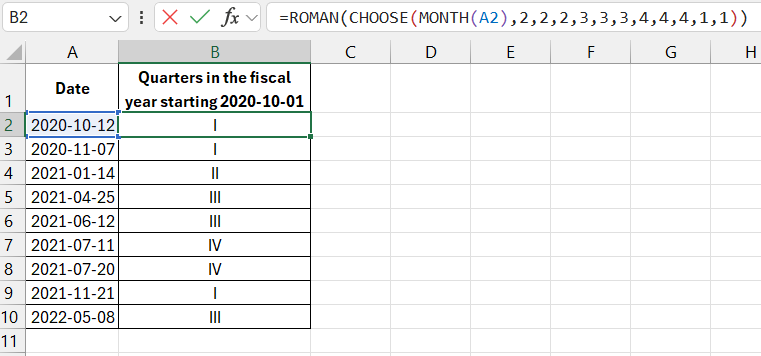
Using the =ROMAN() function, you can enhance the results of the formula by converting Arabic numbers to Roman numerals. The full formula is:
=ROMAN(CHOOSE(MONTH(A2),2,2,2,3,3,3,4,4,4,1,1,1))

In the financial world, quarters are commonly displayed using Roman numerals I-IV.
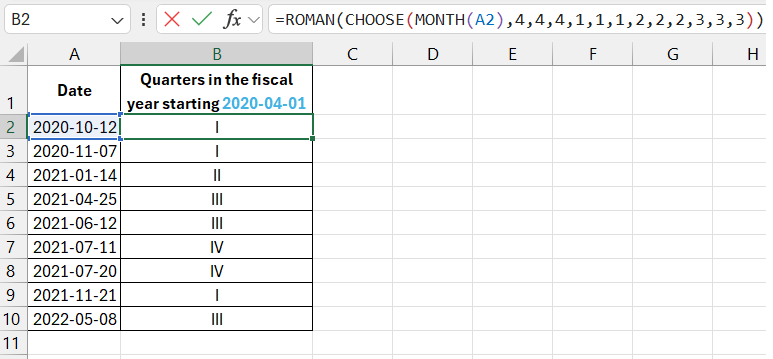
Now, suppose the fiscal year in the company starts in April. The formula would look like this:

Read also: How to Convert Date to Financial Months Using Excel Formula.
It's easy to understand the formula's principle and change the order of quarter numbers in the list according to the order they should appear starting from the month the fiscal period begins. For instance, in the 4th month (4th position in the list), the value should be 1. This means that April is the start of the company’s fiscal year.
Example of the CHOOSE Function in Excel
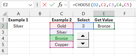
The CHOOSE Function returns a value from a given list based on the specified position number. For example, if you enter the formula =CHOOSE(2,"Gold","Silver","Bronze","Copper") in Excel, you will get "Silver" as the result, since it is in the second position in the list of metals. If you input 4 as the first argument, you'll get "Copper" – the fourth position.

The first (required) argument of the CHOOSE function is the index. This is a number ranging from 1 to the number of values in the list, which is determined by the subsequent function arguments. The maximum number of arguments allowed is 255. The index only specifies which argument should be returned by the function. You can also specify cell references containing the corresponding values in the CHOOSE function arguments:

Download examples of formulas for converting dates to quarters in Excel 
Only the first of the list values must be specified. The remaining 254 arguments complement the list of choices and determine the value returned based on the index. If the index is 1, the first position in the list is returned, if it is 3 – the third position, and so on.
