How to count cells by condition using an Excel formula

Excel offers several functions that perform calculations based on user-defined conditions. Many of them are among the most frequently used Excel functions, such as IF, SUMIF, VLOOKUP, and others. This time, we will look at formulas using the popular COUNTIF function to count the number of values based on a condition.



How to count unique values with a condition in Excel

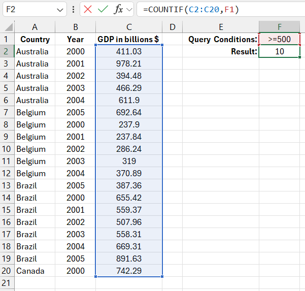
The table below shows the GDP of various countries for 2000–2005. Suppose we need to find out how many times the GDP exceeded 500 billion dollars. This data selection criterion is defined by the condition in cell F1. The formula will look like this:

=COUNTIF(C2:C20,F1)

The COUNTIF function works similarly to the SUMIF function, and its arguments are filled in the same way. The main difference lies in the result: COUNTIF counts the number of values that meet the conditions, while SUMIF sums them.

Another key difference is that COUNTIF lacks the optional third argument found in SUMIF, which allows SUMIF to sum values from a different range of cells than the one that the condition covers. This doesn’t make sense for COUNTIF because counting values in a different range would yield the same result. It's important to note that COUNTIF counts the number of non-empty cells.

In this example, a somewhat non-standard technique is used to fill in the function arguments by simply referencing F1. Traditionally, an ampersand (&) is used to concatenate a comparison operator with a reference to a cell containing a numerical value. For example, ">="&F1, where the cell contains only the number. In this example, the cell already contains a textual value, so the comparison operator is already combined with the value. This approach is acceptable for COUNTIF but incorrect for SUMIF, which would require the second argument to be filled out either as ">="&F1 or ">500".

Alternative formula for conditional cell counting in Excel

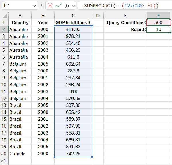
You can also use the SUMPRODUCT function to count cells based on a condition. Below is the formula and illustration:

=SUMPRODUCT(--(C2:C20>=F1))

Download the example formula for counting cells by condition in Excel

The result is the same using another formula.

You may have noticed the double negative in the argument of the SUMPRODUCT function. Inside the parentheses, an array of logical TRUE and FALSE values is created. In Excel, these values can be used in mathematical operations since TRUE=1 and FALSE=0. The negative sign before the parentheses flips the values for arithmetic operations in memory. For example, -(1)=-1. Since we use the double negative, we revert the negative number back to positive, i.e., --(1)=1.

Each TRUE logical value is changed to 1 due to the first negative sign, but it's initially converted to -1. Meanwhile, FALSE is changed to 0. The second negative sign reverts all negative numbers back to positive, and the negative sign has no effect on zero values. Finally, after summing all positive numbers and zeros, we get the correct result returned by the formula.