How to Find the Last Value in the Last Row of Excel Table

When creating formulas in Excel, you often need to find the last row or get the last value in a column of data. There are several conditions to consider before searching: whether the list of values in the column is continuous or contains empty cells, and whether the values are text or numbers. These factors will determine the type of formula to use.



How to Find the Last Non-Empty Row in an Excel Column

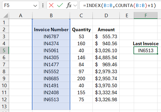
Below is an image of an unsorted list of invoices. Suppose we need to find the last row with an invoice number in the list. A simple way to find the last position in a column is to use the INDEX function combined with counting all positions in the list to determine the last row number.

=INDEX(B:B,COUNTA(B:B)+1)

The INDEX function used with a single column requires only one argument specifying the row number. The third optional argument is not used in this case. The COUNTA function is used to count non-empty cells in column B. The result is incremented by +1, as there is an empty cell in the first row. In this example, the INDEX function returns the 12th row in column B.

The COUNTA function counts cells containing values such as numbers, text strings, dates, and any other values except empty cells. If your data contains empty cells that break the continuity of the lists, this formula will not return correct results.

Finding the Last Number in a Column with Empty Cells in Excel

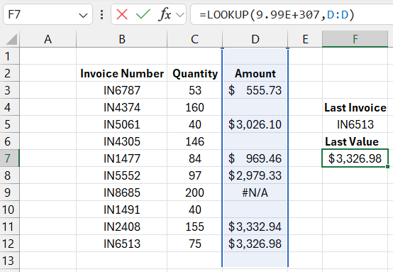
The INDEX and COUNTA functions work well for finding values when the data range does not contain empty cells and is continuous. However, if the data range contains empty cells and the values you are searching for are numbers, you can use the LOOKUP function with a very large number in the arguments. This technique is achieved with the following formula:

=LOOKUP(9.99E+307,D:D)

Download the example of how to find the last value in an Excel table

The value in this formula (a one followed by 308 zeros) is the largest number available in Excel. Since the LOOKUP function has no chance of finding a value larger than the one specified, it stops its calculation at the last numeric value it finds, which is then returned as the result.

What Does a Number with an E in Excel Mean?

A number like 9.99E+307 is written in exponential format. The number before the E is a single digit (0-9) with only two digits after the decimal point. The number after the E indicates how many places to move the decimal point (307 in this example) to get the number written in conventional notation. A plus sign means to shift the decimal point to the right, while a minus sign means to shift it to the left. For example, 4.32E-02 means the number written in decimal form is 0.0432.

The LOOKUP function has the advantage of returning the last number even when the cells in the lookup range might contain not only empty values but also text strings, error codes, or dates.