How to Find the Sum of Numerical and Functional Series

A numerical series is a certain sequence considered together with another sequence (also called a sequence of partial sums). Such concepts are applied in mathematical and complex analysis.

The sum of a numerical series can be easily calculated in Excel using the SERIES.SUM function. Let's look at an example of how this function works, and then we'll plot the function graphs. We'll also learn how to apply the numerical series in practice when calculating capital growth. But first, a little theory.

Sum of a Numerical Series

A numerical series can be viewed as a system of approximations to numbers. The following formula is used to denote it:

Here is the initial sequence of numbers in the series and the summation rule:

∑ - the mathematical sum symbol;
a_i - the general argument;
_i - variable, the rule for changing each subsequent argument;
∞ - the infinity symbol, the "limit" up to which summation is carried out.

The notation Summing the sequence of numbers. means summing natural numbers from 1 to "plus infinity." Since _i = 1, the sum starts from one. If another number (e.g., 2, 3) was here, summing would start from that number (from 2, 3).

According to the variable _i, the series can be written in expanded form:

Summation formula. = а₁ + а₂ + а₃ + а₄ + а₅ + … (up to "plus infinity").

The sum of a numerical series is defined through "partial sums." In mathematics, they are denoted as Sn. Let's express our numerical series in the form of partial sums:

S₁ = а₁

S₂ = а₁ + а₂

S₃ = а₁ + а₂ + а₃

S₄ = а₁ + а₂ + а₃ + а₄

The sum of the numerical series is the limit of the partial sums S_n. If the limit is finite, the series is called "convergent." If infinite, it's called "divergent."

Let's first find the sum of the numerical series:

M = 10.

Now let's build a table of series values in Excel:

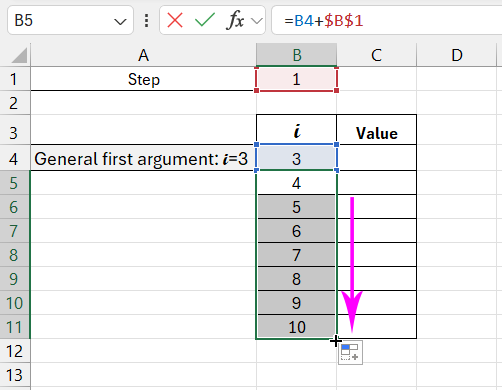
We take the first general argument from the formula: i=3.

All following values _i are found by the formula: =B4+$B$1. Place the cursor at the lower right corner of cell B5 and drag to replicate the formula.

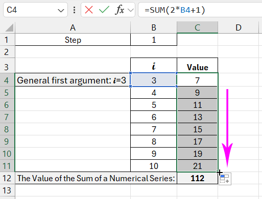
We find the values. Activate cell C4 and enter the formula: =SUM(2*B4+1). Copy cell C4 across the specified range.

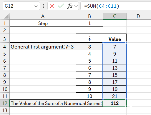
We get the sum of the arguments using the formula: =SUM(C4:C11). The hotkey combination ALT+“+” (plus on the keyboard).

The SERIES.SUM Function in Excel

To find the sum of a numerical series in Excel, the mathematical function SERIES.SUM is used. The program uses the following formula:

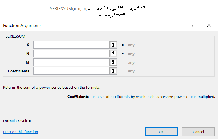
The function's arguments:

x – the variable value;
n – the degree for the first argument;
m – the step by which the degree of each subsequent term increases;
a – the coefficients for the corresponding degrees of x.

Important conditions for the function to work:

all arguments are mandatory (i.e., all must be filled in);
all arguments are numerical values;
the coefficient vector has a fixed length (the infinity limit won't work);
the number of "coefficients" = the number of arguments.

Calculating the Sum of a Series in Excel

The same SERIES.SUM function works with power series (one type of functional series). Unlike numerical series, their arguments are functions.

Functional series are often used in finance and economics. You could say this is their applied area.

For example, suppose you deposit a certain amount of money (a) in a bank for a certain period (n). You receive an annual interest rate of x percent. To calculate the accumulated amount at the end of the first period, the formula is:

S₁ = a (1 + x).

At the end of the second and subsequent periods, the expression looks like this:

S₂ = a (1 + x)²; S₃ = a (1 + x)² and so on.

To find the total sum:

S_n = a (1 + x) + a (1 + x)² + a (1 + x)³ + … + a (1 + x)ⁿ

Partial sums in Excel can be found using the FV() function.

Initial parameters for the task:

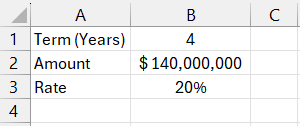
Using the standard mathematical function, we find the accumulated sum at the end of the term. To do this, enter the formula in cell D2: =B2*POWER(1+B3,4)

Now in cell D3, we solve the same task using Excel's built-in function: =FV(B3,B1,,-B2)

The results are identical, as expected.

How to fill in the FV() function arguments:

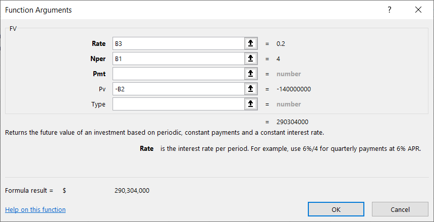
"Rate" – the interest rate for the deposit. Since cell B3 is formatted as a percentage, we simply referenced that cell in the argument field. If it were a number, we would write it as a fraction (20/100).
"Nper" – the number of periods for interest payments. In our example, it’s 4 years.
"Pmt" – periodic payments. In our case, there are none, so we leave this argument blank.
"Pv" – "present value," the deposit amount. Since we are parting with this money temporarily, we enter it with a minus sign.

Thus, the PV function helped us find the sum of the functional series.

Excel also has other built-in functions for finding different parameters. These are usually functions for working with investment projects, securities, and amortization payments.

Plotting the Function Graph for the Sum of a Numerical Series

Let’s plot the function graph reflecting capital growth. To do this, we need to plot the function, which is the sum of the built series. For example, we’ll take the same deposit data:

Next, we need a function for compound interest - FV(). We will find the future value of investments with equal payments and a constant interest rate. Using the FV() function, we will fill in the table:

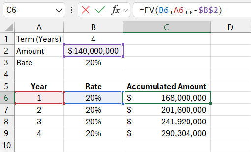
In the first row, we see the accumulated sum after one year. In the second row—after two years, and so on.

Let's add another column where we show the profit:

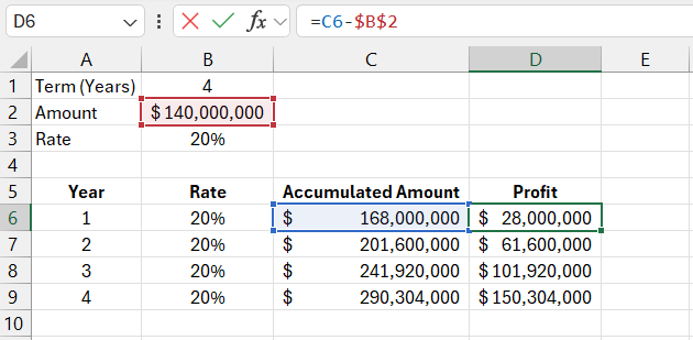
Here's how we calculated it—in the formula bar.

Based on the obtained data, we'll create a function graph.

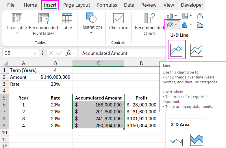
Select two ranges: C5:C9. Go to the "Insert" tab, then to "Charts" tools. Select the first chart:

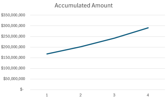
Let's make the task even more "applied." In the example, we used compound interest, which is added to the amount accumulated in the previous period.

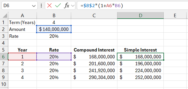
For comparison, let's use simple interest. The formula for simple interest in Excel: = $B$2*(1+A6*B6)

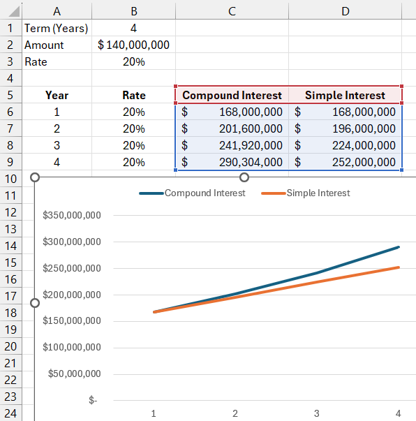
We will add the obtained values to the "Capital Growth" chart.

Chart with compound and simple interest.

Download example on how to find sum of numerical and functional series download file

The conclusions that the investor would draw are clear.

The mathematical formula for the partial sum of a functional series (with simple interest): S_n = a (1 + x*n), where a is the initial deposit amount, x is the interest rate, and n is the period.