How to get Present Value of Investments and Money in Excel
The Time Value of Money (TVM) is an important concept in accounting and finance. The idea is that a ruble today is worth less than the same ruble tomorrow. The difference between these two financial values is the profit that can be gained from one ruble or the loss. For example, this profit can be earned from interest accrued on a bank account or as dividends from investments. But there can also be a loss when paying interest on debt repayment.
Example of Calculating the Discounted Present Value of Investments in Excel
Excel offers several financial functions to calculate the time value of money. For example, the PV (present value) function returns the current value of investments. Simply put, this function reduces the amount by the discount rate and returns the present value for that amount. If an investment project is expected to bring in a profit of 10,000 in a year, the question is: what is the maximum amount you should risk to invest in this project?
For example, in Russia, retail businesses sometimes make up to 35% profit annually, while wholesale businesses no more than 15%. Given the small investment amount, it is assumed that the investment object is not a wholesale business, so a profit greater than 15% annually should be expected. Below is an example of the investment return calculator formula in percentages:
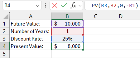
=PV(B3,B2,0,-B1)

As we see in the image, the calculator shows that to receive 10,000 in 1 year with a 25% return, we need to invest 8,000. In other words, if we had 8,000 and invested it at 25% annually, we would earn 10,000 in a year.
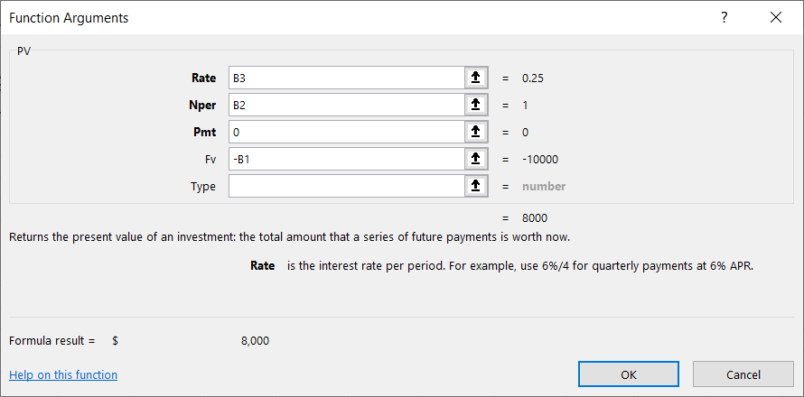
The PV function has 5 arguments:

- Rate – the discount rate. This is the percentage of profit that can be expected during the discounting period. This value has the greatest impact on calculating the present value of investments, but it is the hardest to determine accurately. Cautious investors usually underestimate the rate to the maximum realistically achievable level under certain conditions. If the funds are intended for loan repayment, this argument is easily determined.
- Number of periods (Nper) – the period of time during which the future amount is discounted. In this example, 1 year is indicated (recorded in cell B2). The interest rate and the number of years should be expressed in corresponding units of measurement. This means that if you use an annual rate, then the number in this argument means the number of years. If the rate in the first argument is monthly (for example, 2.5% monthly), then the number in the second argument means the number of months.
- Payment (Pmt) – the amount that is periodically paid over the discount period. If only one payment is provided, as in the example above, this amount is the future value of the money, and the payment itself equals 0. This argument must be consistent with the second argument, the number of periods. If the number of discount periods is 10 and the third argument is not equal to 0, the PV function will calculate it as 10 payments in the amount specified in the third argument (Pmt). Below is another example of how the present value of money is calculated with multiple separate payments.
- Future Value (FV) – this is the amount that should be received at the end of the discount period. Excel's financial functions are based on cash flow calculations. This means that the future value and the present value of investments have opposite signs. In this example, the future value is a negative number, so the formula returns a positive number.
- Type – this argument should be 0 if the payment of the final amount falls at the end of the discount period or 1 if it is at the beginning. In this example, the value of this argument does not matter and will not affect the final calculation. Since the payment is 0, this argument can be omitted, and the function will default to assigning a value of 0.
Formula for Calculating the Present Value with Inflation in Excel
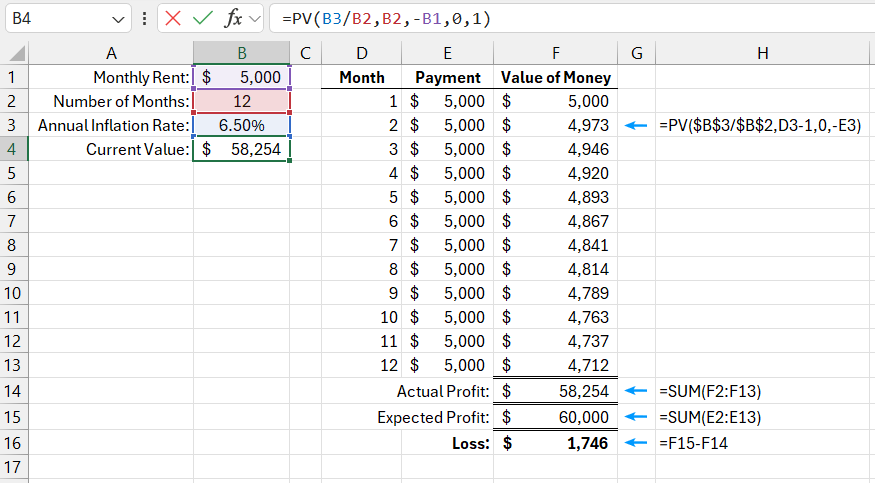
In another example of using the PV function, the future value of money is calculated for a series of equal future payments. If, for instance, under an office lease agreement, the tenant must pay 5,000 each month for one year, the landlord can use the PV function to calculate how much income they will lose, considering 6.5% annual inflation:
=PV(B3/B2,B2,-B1,0,1)

Download example How to Calculate Present Value of Investments and Money in Excel 
In this example, the fifth argument "Type" has a value of 1, as the rent is paid at the beginning of each month.
In the case of regular payments, the PV function calculates the present value of money separately for each payment and sums the results. The image shows the calculated values for each payment. The present value of the first payment is the same as the payment itself because it is paid now. The payment in the next month will be made in one month, and its present value is already reduced (depreciated). It is discounted to 4,973. The changes are minor, but the last payment, which will be made in 11 months, has a significantly lower value of 4,712. All present values of investment must be summed up. The PV function does all this work automatically without the need to create a chronological payment schedule for the entire period.
