How to make Loan Calculator Floating Interest Rate in Excel
There are loans with a floating interest rate. How do you create a payment schedule for a loan with a variable interest rate? The discounting of such loans often depends on official financial indices. For example, LIBOR (London Interbank Offered Rate) when raised by a certain percentage is often described as: “LIBOR +3%”. Let's look at a specific example.
Loan Calculator with a Floating Interest Rate in Excel
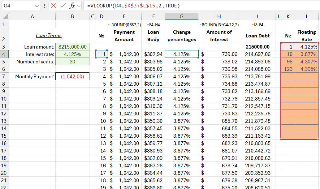
Below is an image of a payment schedule for a loan with a floating interest rate. It contains a "Rate Change" column that clearly shows the fluctuation of the interest rate. In a separate table, the variable interest rates are recorded.
The formula in the "Rate Change" column substitutes the corresponding interest rates from the additional table based on a condition:
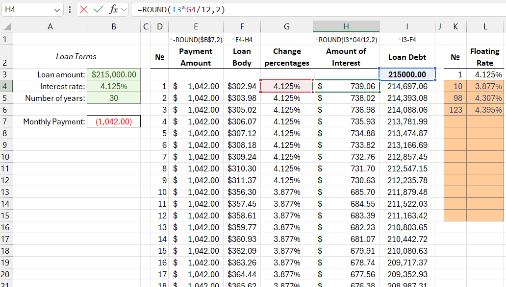
The formula in the "Interest Amount" column uses data from the cells in the "Rate Change" column:
Note: All formulas in each column are shown above the column headers, except for column G, where the formula is: =VLOOKUP(D11;$K$11:$L$23;2;TRUE).
In the "Rate Change" column, the VLOOKUP function is used, where the fourth argument is set to TRUE. To use this argument, the data in the first column of the additional table with floating interest rates must be sorted in ascending order. The VLOOKUP function finds the closest larger value in the first column of the additional table for each current payment number in the main table. The function doesn't require an exact match but instead looks for the nearest larger value corresponding to the number from the first column of the additional table. Once the nearest larger value is found, the VLOOKUP function returns the interest rate from the cell next to the found number. For example, when the function searches for the interest rate for payment number 16, it returns the value from the second row, as the nearest larger value than 16 in the next row is 98. Thus, 98 is the closest larger number to the sought number 16.
Loan Payment Schedule with a Floating Interest Rate in Excel
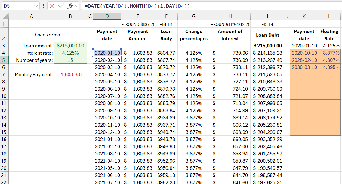
In loan payment schedules, dates are usually used instead of payment numbers. To replace the payment numbers with dates in the schedule, follow these steps:
- In cell D4, enter the date of the first payment (for example: 01/10/2020).
- In cell D4, enter a formula, which should be copied into the other lower cells of column D (now labeled "Payment Date" instead of "No."):
- In column K "Payment Date" in the additional table with interest rates (range: K2:L15), enter the dates from which the interest rate will change in the loan payment schedule.
=DATE(YEAR(D4),MONTH(D4)+1,DAY(D4))
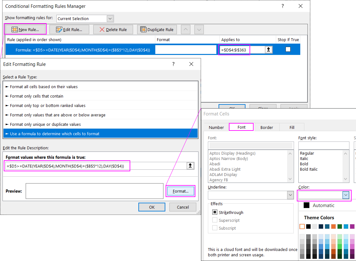
You should also create conditional formatting to automatically hide cells with negative loan balances when the loan term is shortened. For example: instead of 30 years, 20 years. By changing the font color to white, we can hide unnecessary values in the schedule according to the condition. To do this, select the range of the table part of the schedule D4:I363 and choose the tool: "HOME"-"Styles"-"Conditional Formatting"-"Create Rule".
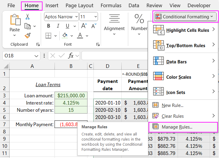
In the "New Formatting Rule" window that appears, select the option "Use a formula to determine which cells to format" and enter the formula in the "Edit the Rule Description" field:
=$D5>=DATE(YEAR($D$4),MONTH($D$4)+($B$5*12),DAY($D$4))
Download Loan Calculator with Floating Interest Rate in Excel 
Then click the format button and set the font color of the cell values to white.
As a result, the payment schedule dynamically hides unnecessary negative values when the loan term is shortened in the condition parameters of the first table on the left.

Data Visualization Charts for Interactive Report Creation in Excel.
Dashboard Templates