How to make a Loan Repayment Schedule Calculator in Excel
The main indicator in a loan repayment schedule is the amount of the monthly payment. To calculate the monthly payment amount in Excel, you can use the PMT function. Instead of inputting specific values directly into the function, such as the loan amount and interest rate, you can enter these values into separate cells and reference them in the PMT function arguments. This allows you to easily adjust the loan terms and see their impact on the monthly payment. This way, you can create a loan calculator and generate a payment schedule in Excel.
How to Create a Loan Calculator in Excel
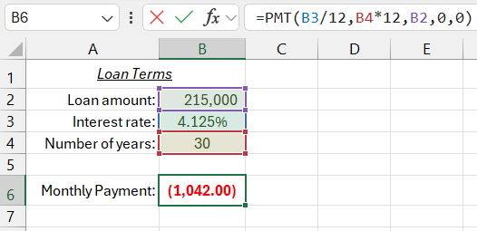
Below is an example of a simple loan calculator in Excel that calculates how much you will need to pay the bank monthly to repay the loan. The user should enter the relevant loan terms into cells B2:B4, and the result of the PMT function will be displayed in cell B6. The monthly payment for the loan is calculated with the following formula:
=PMT(B4/12,B5*12,B3,0,0)

The PMT function has 3 required arguments and 1 optional:
- Rate – the nominal annual interest rate divided by the number of capitalization periods in a year. In this example, the loan is capitalized monthly, so the interest rate specified in cell B3 is divided by 12 (months).
- Number of periods – the total number of payments over the life of the loan. In other words, the user of the loan calculator must enter the number of years of the loan, and payments will be made monthly. Therefore, the number of years specified in cell B4 is multiplied by 12 (months).
- Present value – the current loan balance. Excel functions for loan calculations, including the PMT function, are based on cash flow calculations. If the current loan value and payment amounts are considered cash inflows and outflows, it is easy to understand why and when these functions' results will be positive or negative numbers. In this example, the bank lent you $215,000, so this amount is considered a cash inflow for you (a positive value). The result of the PMT function is negative because monthly loan payments are considered an outflow for you.
- Type – specifies whether payments are made at the beginning (1) or end (0) of the period.
Note: If the PMT function should return a positive number, you can enter a negative number for the present value argument. In this case, the calculation is done from the bank's perspective: the loan is an expense, and loan payments with interest are cash inflows for the bank.
A common mistake in financial formulas is confusing capitalization periods with payment frequencies. In this example, the annual interest rate is divided by 12 to compute the monthly interest rate for capitalization. At the same time, the number of periods is multiplied by 12, as payments are made monthly. Both arguments must be adjusted to monthly periods for capitalization and payments to ensure the correct result.
If the user forgets to divide the discount rate by 12, Excel would assume the entered value as monthly discounting, resulting in a much higher payment. Similarly, if the number of payments is entered as the number of years with monthly discounting, Excel would assume payments are made annually.
The PMT function does not inherently know what the entered number represents – years, months, or days. It assumes that the discount rate and number of years refer to the same period.
How to Create a Loan Payment Schedule in Excel
Once the loan payment amount is calculated, you can create a loan payment schedule that includes information on the portion of each payment that goes towards the principal and interest, as well as the remaining loan balance after each payment.
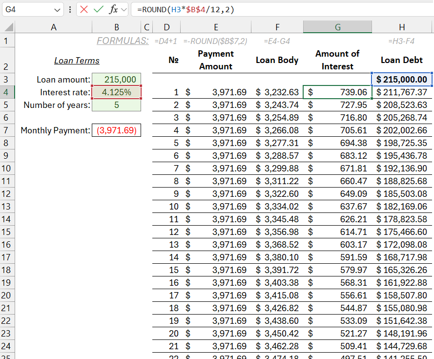
Below is a fragment of a payment schedule. It consists of the following columns:
- Number – the sequential number of the current loan payment. Enter the number 1 in cell D4, and in the next cell D5, enter the formula =D4+1 and copy it down to D363 (this schedule will contain 360 payments).
- Payment amount – calculated using the PMT function in cell =$B$7 and rounded to the nearest cent. Although Excel performs calculations with many decimal places, the schedule should show amounts rounded to cents. This means that at the end of the loan term, a small amount may remain for settlement with the bank. Enter the formula =-ROUND($B$7,2) in cell E4 and copy it down to E636.
- Principal – the portion of the payment that reduces the loan balance excluding interest. Enter the formula =E4-G4 in cell F4 and copy it down to F363.
- Interest amount – the portion of the payment representing interest charged on the loan. This column shows how much the bank earns each month from the loan, that is, its gross profit from lending. The loan balance after the previous payment is multiplied by the annual interest rate and divided by 12. The result is rounded to the nearest cent. Enter the formula =ROUND(H3*$B$4/12,2) in cell G4 and copy it down to G363.
- Remaining balance – the remaining loan balance after each payment. Enter the formula =B3 in cell H3, which returns the initial loan amount. Enter the formula =H3-F4 in the other cells of this column. It reduces the loan balance by the principal portion of each payment. The interest portion is kept by the bank.

The example shown in the second image has a loan term of 15 years, while the first image shows a 30-year term. Reducing the loan term increases the monthly payment amount.
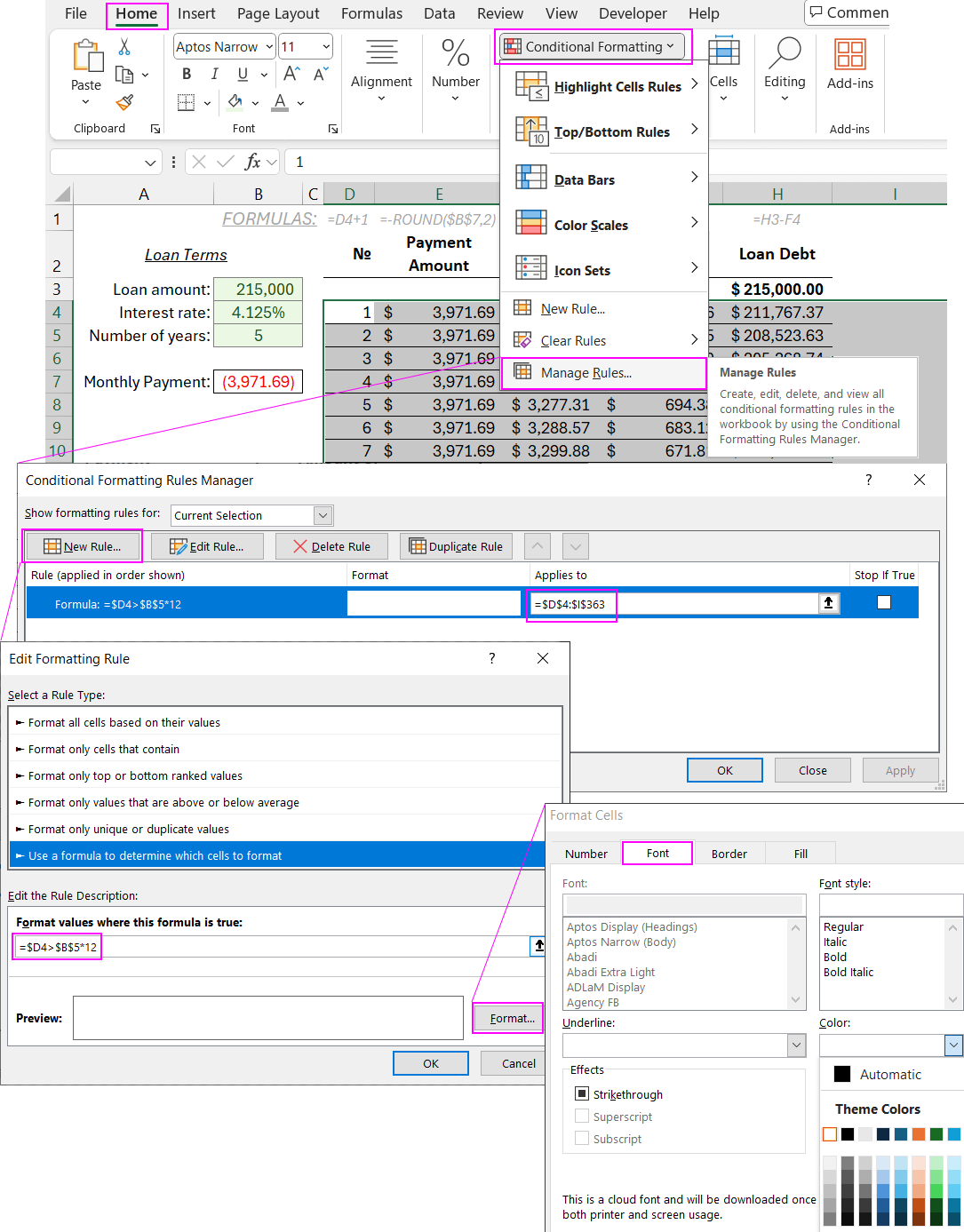
The final step involves hiding cells with negative values in the loan repayment schedule. This applies to the calculator rows until the end of the loan term. If a different loan term is specified, such as 10 years instead of 15 or 30 years, extra calculation results will be hidden. This can be achieved using conditional formatting, which will change the font color of the relevant cells to white. By setting the font color to white on a white background, unnecessary data can be easily hidden.
To do this, select the range D4:H363 and choose the tool: "HOME" - "Styles" - "Conditional Formatting" - "Create Rule."
The formula used in conditional formatting is shown in the image below:

Download Example How to Create Loan Repayment Schedule in Excel 
This formula compares the current payment number in column D with the number of years specified in cell $B$5 multiplied by 12. If the payment number exceeds this value, the formula returns TRUE and applies the white font color. If the payment number is less than or equal to the total number of payments, no formatting changes are applied to this group of cells.
