How to Make a Selection in Excel Using Array Formulas
Excel provides tools to make selections of specific data from a range, whether at random, based on one condition, or several. These tasks are generally solved using array formulas or macros. Let’s look at some examples.
How to Make a Selection in Excel Based on a Condition
When using array formulas, selected data is displayed in a separate table, which is the advantage of this method over a standard filter.
Source table:
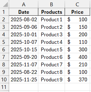
First, let’s learn how to make a selection based on one numerical criterion. The task is to select items from the table priced above 200 rubles. One way to do this is by using filtering, which leaves only the items that meet the condition in the original table.
Another method is to use an array formula. The rows that meet the condition will be placed in a separate report table.
First, create an empty table next to the source table: duplicate the headers, and keep the same number of rows and columns. The new table will occupy the range E1:G10. Now, select E2:E10 (the "Date" column) and enter the following formula: {
=IFERROR(INDEX($A$2:$A$10,SMALL(IF(200<=C2:C10,ROW($C$2:$C$10),""),ROW()-ROW($C$1))-ROW($C$1)),"")}.
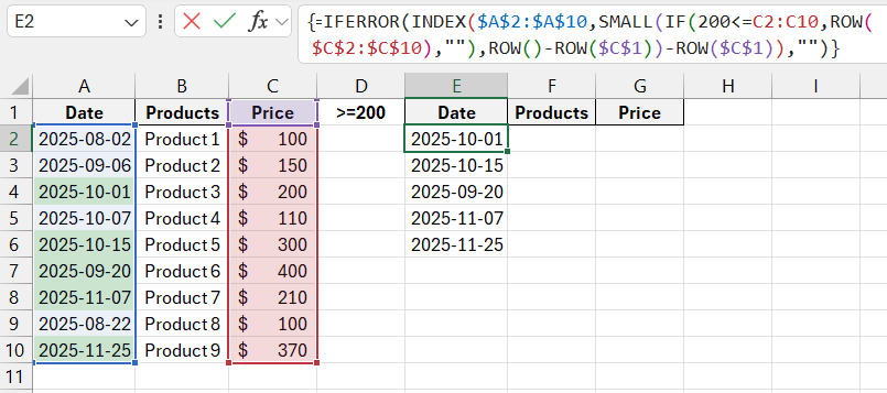
To make this an array formula, press Ctrl + Shift + Enter. Enter a similar array formula for the next column, "Product": {
=IFERROR(INDEX($B$2:$B$10,SMALL(IF(200<=C2:C10,ROW($C$2:$C$10),""),ROW()-ROW($C$1))-ROW($C$1)),"")}. Only the first argument of the INDEX function has changed.
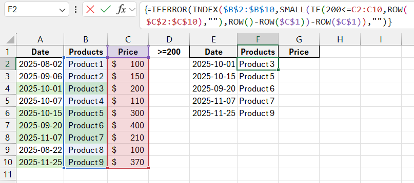
For the "Price" column, use the same array formula but change the first argument of the INDEX function.
The result is a report on products priced above 200 rubles.
=IFERROR(INDEX($C$2:$C$10,SMALL(IF(200<=C2:C10,ROW($C$2:$C$10),""),ROW()-ROW($C$1))-ROW($C$1)),"")
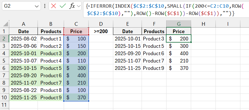
This selection is dynamic: when the request changes or new items appear in the source table, the report will automatically update.
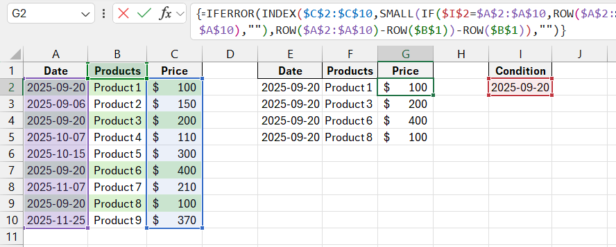
Task #2 – Select items that went on sale on 20.09.2015. In this case, the selection criterion is a date. For convenience, we’ll enter the target date into a separate cell, I2.
An array formula similar to the one used previously is used to solve this problem. The difference is that the condition uses the equals sign instead of <=: {
=IFERROR(INDEX($C$2:$C$10,SMALL(IF($I$2=$A$2:$A$10,ROW($A$2:$A$10),""),ROW($A$2:$A$10)-ROW($B$1))-ROW($B$1)),"")}.
Similar formulas are entered into other columns (see the principle above).
Now, let’s use a text criterion. Instead of a date, enter the text “Product 1” in cell I2. The array formula is slightly modified: {
=IFERROR(INDEX(C$2:C$10,SMALL(IF($I$2=$B$2:$B$10,ROW($B$2:$B$10),""),ROW($B$2:$B$10)-ROW($B$1))-ROW($B$1)),"")}.
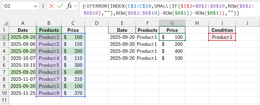
This large Excel selection function can handle both numerical and text-based criteria.
Selection Based on Multiple Conditions in Excel
Task: Select products priced between 200 and 400 rubles. Combine the conditions using the “*” symbol. The array formula looks like this: {
=IFERROR(INDEX(A$2:A$10,SMALL(IF(($I$2<=$C$2:$C$10)*($I$3>=$C$2:$C$10),ROW($C$2:$C$10),""),ROW($C$2:$C$10)-ROW($C$1))-ROW($C$1)),"")}.
This formula is for the first column of the report table. For the second and third columns, change the first argument of the INDEX function. The result:
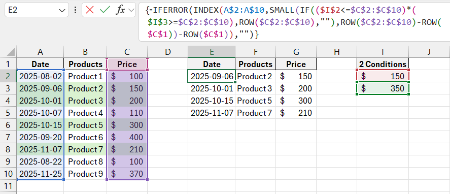
To make a selection based on multiple dates or numerical criteria, use similar array formulas.
Random Selection in Excel
When working with large datasets, a random selection may be required for further analysis. Each row can be assigned a random number, then sorted for selection.
First, insert an additional column on the left. In cell A2, enter the formula RAND(). Drag it down the entire column:
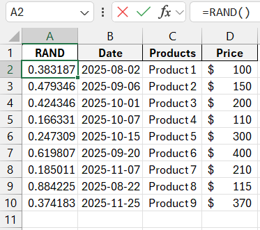
Now, create a formula for the selection table of random values from the source data:
=INDEX(D$2:D$10,MATCH(LARGE($A$2:$A$10,$H$1),$A$2:$A$10,0))
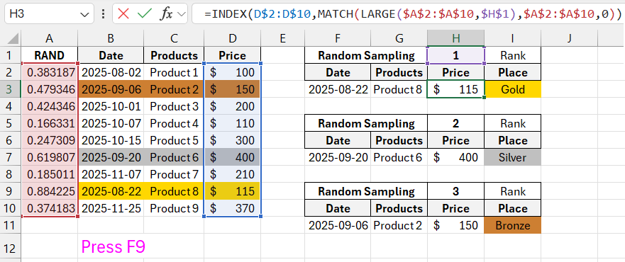
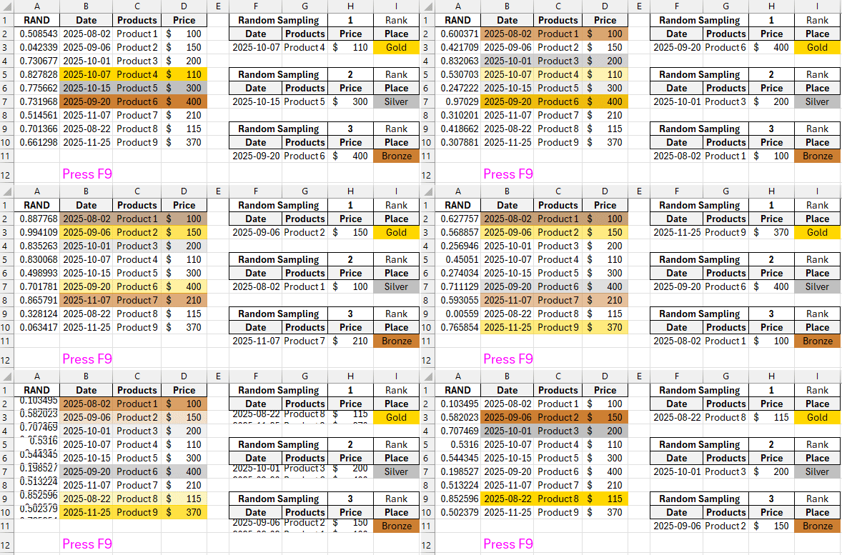
By periodically pressing F9 on the keyboard, the random selection of data will automatically refresh.

Download Example Formulas for How to Make Selection in Excel 
Thanks to the use of the LARGE function, we can simultaneously obtain 3 non-overlapping random values.
