How to Select All Matching Values in an Excel Table
One of the limitations of the VLOOKUP function and other lookup functions in Excel is that they find only the first matching value based on the search query in the data list. But what if the table contains multiple matching values that meet the user's request? To find the second, third, or subsequent matching values, you need to use an array formula.
How to Find All Matching Values in a Column in Excel
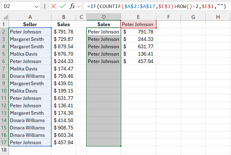
Below is an image showing a list of sellers and their sales figures. The names of some sellers are repeated in the list. Next to the original table is a filtered list containing all sales results for a specific seller. To create such a query list from the original table, using the VLOOKUP function alone is insufficient because this function only finds and returns the first match. However, in this case, we need to get all the values that match the query and display them in a separate list. The first formula:
=IF(COUNTIF($A$2:$A$17,$E$1)>ROW()-2,$E$1,"")

The formula used in column D is simpler. It returns a list where the seller's name appears as many times as it does in the original table. The COUNTIF function is used to determine how many times the name is repeated.
The formulas in columns D and E are copied to the other cells below to display all matching values.
The formula in column D returns the name entered in cell E1 if the number of occurrences of the seller's name in the original table is greater than the result of the ROW()-2 formula. In the first cell of the original table, A2, the ROW()-2 formula returns 0. Since the name "Zasyadko Petr" appears more than 0 times in the list, it is displayed in the list on the right. However, in the sixth row of the sheet, the ROW()-2 formula returns 5, which equals the number returned by the COUNTIF($A$2:$A$17;$E$1) formula. In this case, an empty string ("") is returned. In the next row (7), ROW()-2=6, which is greater than 5, so again, an empty string is returned instead of a name, and so on.
How to Select All Matching Values in a Column in Excel
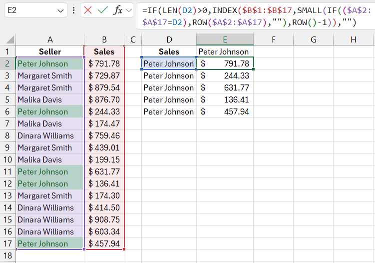
The formula in column E is an array formula that requires pressing CTRL+SHIFT+Enter to input. This formula first checks whether the name is in the adjacent cell in column D. If the cell is empty, it returns an empty string. In the first case, the INDEX function is used to return the sales corresponding to the current number of name repetitions in the original table. The second formula:
=IF(LEN(D2)>0,INDEX($B$1:$B$17,SMALL(IF(($A$2:$A$17=D2),ROW($A$2:$A$17),""),ROW()-1)),"")

Download example of formula for selecting all matching values in Excel 
The above formula performs several functions, specifically INDEX, SMALL, and ROW. The SMALL function looks for the row with the smallest value, which is passed as an argument to the INDEX function, returning the value found in that row.
The "Row Number" argument in the INDEX function uses the SMALL function. Its first argument is a table (in this case, a table of rows or empty values), and the second argument is a number defining the ordinal number of the smallest value. For example, the number 2 in the second argument causes the function to return the second smallest value. The second argument uses the ROW-1 formula, which acts as a counter for the ordinal numbers of the smallest values. The number 1 is subtracted because the data in the original table is recorded starting from the second row. The formula in the second row of the Excel worksheet returns the first smallest value, and in the third row, the second smallest value, and so on.
The SMALL function ignores text strings and operates only with numbers. To get the row number of a cell in the range A2:A17 containing the original seller names, you need to use the IF function. If the current name does not match the desired seller name, an empty string will be returned, which the SMALL function simply ignores. When the IF function uses the desired name, "Zasyadko Petr," the numeric value table is passed to the SMALL function. This is how the array table looks schematically in the program's memory:
{2;"";"";"";6;"";"";"";"";11;12;"";"";"";"";17}
This array table consists of 16 elements. When the checked cell contains the name "Zasyadko Petr," the current row number of that cell is added to the table, and the SMALL function returns the smallest number in order. For example, in the fourth formula in cell E5, this function returns the number 12, which is the fourth non-empty element in the array. At the same time, the INDEX function returns the value from the adjacent cell in that row, 136.41.
What Is an Array Formula in Excel
Array formulas are special formulas that work with arrays of numbers. A regular formula is entered by pressing the Enter key once. To input an array formula, press Enter while holding down CTRL and SHIFT. As mentioned, the key combination is CTRL+SHIFT+Enter.
To ensure that an array formula is used in a cell, check the formula bar. Excel places array formulas in curly braces. There is no point in manually entering these curly braces, as it will not work. Only the key combination will work!
It is worth noting that some functions, such as SUMPRODUCT, work similarly to array formulas but do not require the key combination because they are regular formulas. SUMPRODUCT calculates only the sum of values in data arrays. If you need to perform other operations on data arrays, such as using functions like SMALL or AVERAGE, you must use an array formula with these functions, remembering to press CTRL+SHIFT+Enter to input it!
