How to Use CHOOSE Formula with Multiple Conditions in Excel
The CHOOSE function is perfect for using multiple formulas in a single cell simultaneously. This allows the user to switch between formulas and select the one that should be executed.
Examples of Selecting Formula Execution Based on User Conditions
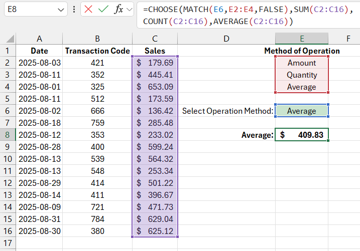
The image below shows a sales report and three ways to aggregate data. For convenience, a dropdown list is created, from which the user selects the aggregation method:
=CHOOSE(MATCH(E6,E2:E4,FALSE),SUM(C2:C16),COUNT(C2:C16),AVERAGE(C2:C16))
Syntax of the CHOOSE function:
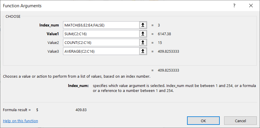
The first argument of the CHOOSE function is called "Index Number" and determines which of the subsequent arguments should be returned through the function. This argument can take numerical values from 1 to the maximum number of subsequent arguments, up to 254. The following 254 arguments contain the values that the function will return. If the "Index Number" argument contains the number 1, the function will return the content of the second argument. And if the index number is 2, the third argument will be returned, and so on.
The subsequent arguments after the first "Index Number" are called "Value1"; "Value2"... "Value254". In the formula above, they define 3 ways to aggregate sales data that the user can select:
- The SUM function – sums the numbers in a range of cells.
- COUNT – counts the number of non-empty cells with numbers.
- AVERAGE – returns the arithmetic mean for the range of numbers in the cells.
The value in the first argument of the CHOOSE function is calculated by the MATCH function, which in this example returns the number 1, 2, or 3 depending on which position in the dropdown list the user selects in cell E6:
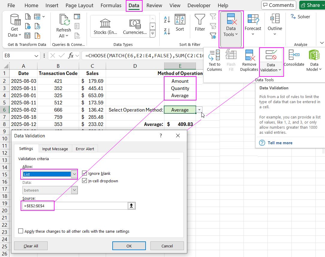
The dropdown list itself is filled with values by referencing the range of cells E2:E4.
If the user selects the "Sum" option from the dropdown list, the MATCH function will return the number 1 as a result of the calculation for the first argument of the CHOOSE function. As a result, the entire formula will return the result of the SUM function, which is in the second argument. If the user selects the "Count" option, then MATCH will return the number 2, and the entire formula will return the result of COUNT from the third argument.
As shown in the image above, the user selected the "Average" option, so the MATCH function returned the number 3, and then CHOOSE executed the AVERAGE function from the fourth argument. As a result, the entire formula returned its average value.
Example of Using the SUBTOTAL and CHOOSE Formulas in Excel
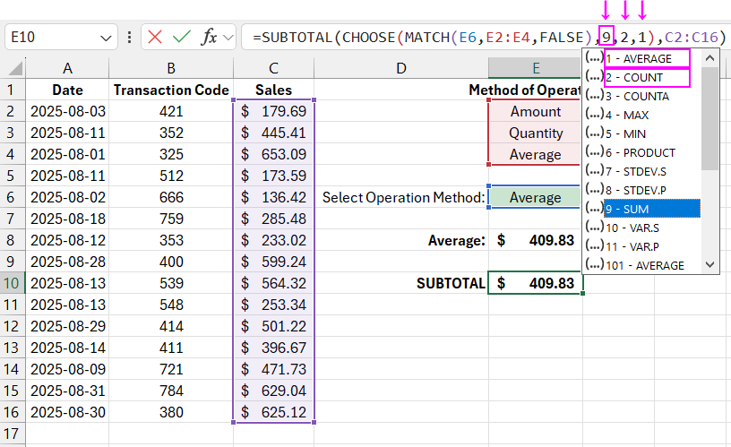
An alternative way to apply the CHOOSE and MATCH functions in formulas is to use them together with the SUBTOTAL function. This function is very versatile and allows several data aggregation methods to be applied to the same range of cells. When the first argument of the SUBTOTAL function contains the value 1, the arithmetic mean of the numbers in the same cell range is displayed:
=SUBTOTAL(CHOOSE(MATCH(E6,E2:E4,FALSE),9,2,1),C2:C16)
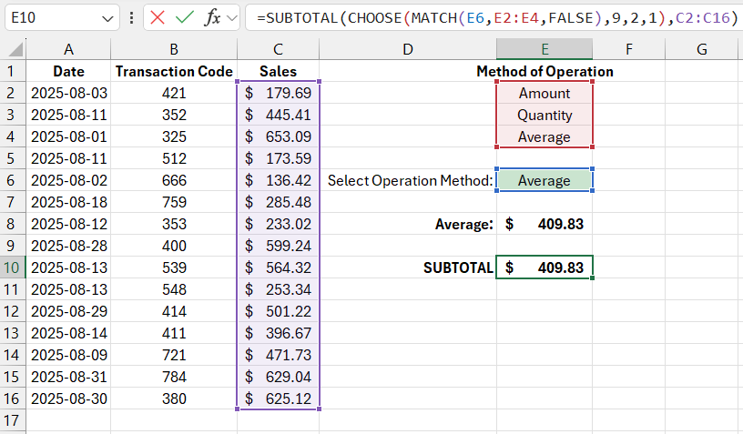
For example, if the first argument of the SUBTOTAL function is equal to the number 9, the values in the range of cells will be summed. If the first argument is 2, then the number of cells in the same range will be counted:
Download example How to Use CHOOSE Formula with Multiple Conditions in Excel 
Inside the SUBTOTAL function, you can use the CHOOSE and MATCH functions to determine the method of data aggregation. This method of composing the formula is more restrictive than simply placing formulas inside the CHOOSE function. After all, the number of data range processing methods by the SUBTOTAL function is limited to 22.
