How to use COUNTIFS formula - multiple conditions in Excel
The COUNTIF function has a related function in Excel – SUMIF. Naturally, Excel developers wouldn't create the SUMIFS function for summing values with multiple conditions without also developing the COUNTIFS function for counting cells based on multiple criteria.
COUNTIFS formula for counting cells with multiple conditions in Excel
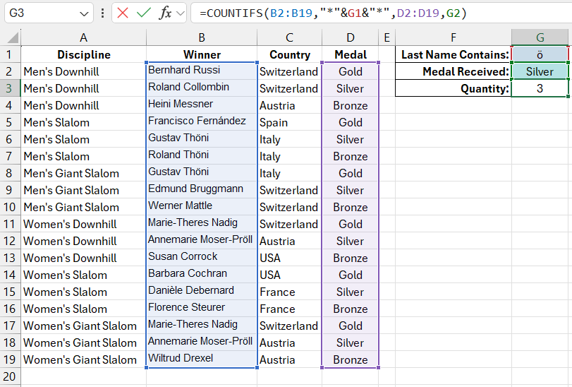
Below is a table of medalists from the 1972 Winter Olympics in alpine skiing. In this example, we need to find how many silver medalists have the letter "ö" in their last name. The letter to search for is recorded separately in cell G1, and the medal type is in cell G2. The formula is as follows:
=COUNTIFS(B2:B19,"*"&G1&"*",D2:D19,G2)

The COUNTIFS function requires arguments to be filled in pairs Range_1;Criteria_1, similar to the syntax of the SUMIFS function (except SUMIFS has one extra argument – Sum_Range).
The first argument in the COUNTIFS function is Range_1. It specifies the cell range B2:B19, which contains the list of medalists' last names. The second argument – Criteria_1 consists of a combined string of wildcard characters and a reference to the cell between them "*"&G1&"*". The string is assembled using the concatenation operator – &. The asterisks on both sides of the reference indicate that the match does not have to be exact. Any characters in any quantity are allowed before and after the required fragment, in this case, the letter "ö". Blank strings are also acceptable. This combination in the criteria allows for considering all values in the checked string. Therefore, there's no need to worry if the letter is not at the beginning or end of the last name but appears somewhere in between.
The third argument, Range_2 (the first in the second pair of arguments), reads the values in the range D2:D19 containing the string "Silver" (as specified in cell G2). This way, it counts only those cells that meet the conditions in both pairs of arguments of the COUNTIFS function. In this example, the last names of the silver medalists with the letter "ö" are: Gustav Thöni, Annemarie Moser-Pröll, and Annemarie Moser-Pröll again. A total of 3 medalists meet the selection criteria from the table.
Another formula for counting values based on multiple conditions
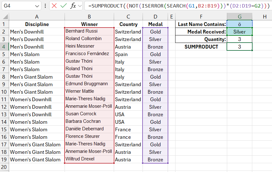
The COUNTIFS function is relatively new, first appearing in Excel 2010. If you're using an older version of Excel or opened a file from an older version, SUMPRODUCT might have been used instead of COUNTIFS. It was commonly used for counting cells based on multiple conditions or solving similar tasks. Thus, this old function will still be supported in newer Excel versions. For instance, the same task can be solved with an alternative formula:
=SUMPRODUCT((NOT(ISERROR(SEARCH(G1,B2:B19)))*(D2:D19=G2)))

Download an example of how to use the COUNTIFS formula with multiple conditions in Excel 
In the end, we get the same result, although this formula is less readable.
The value defined by the condition on the left of the asterisk will be converted into a logical array of TRUE or FALSE values. Similarly, the value on the right of the asterisk will be determined. Logical values in Excel are often used in mathematical operations, where TRUE=1 and FALSE=0. If the value on the left and right table is 1, the formula multiplies these two ones together 1*1=1 and passes the result (the number 1) to the root function for summation. But if any of the arrays return a FALSE value = 0, then the number 0 is passed for summation. The SUMPRODUCT function adds all the returned numbers and provides their total sum, which is the result of the entire formula. Ultimately, we get the number of rows that meet the multiple conditions.
In the second array to the right of the asterisk, the condition is fairly easy to read: (D2:D19=G2). Each value in the range D2:D19 must equal the value in cell G2. If so, TRUE is entered into the table, otherwise – FALSE.
However, the first array to the left of the asterisk is quite complex in syntax. As you know, the result of the condition check must be a set of logical TRUE and/or FALSE values. To achieve this, you need to correctly construct a logical expression that returns such values. The FIND function first searches for the letter "ö" in the current cell. The address of the range where the search is performed, as well as the letter itself, are specified in its arguments. The FIND function returns the position number of the target letter in the current string. For example, the formula =FIND("ö","Thöni") returns the number 3, as the letter "ö" is the third character in "Thöni". If the letter is not found, the formula returns an #ERROR! However, we don't need error values, only logical TRUE or FALSE.
The ISERROR function helps handle error values, returning only TRUE or FALSE, accepting errors. We're getting closer to our goal, but the problem is that TRUE will be returned if the FIND function does not find the letter "ö" in the current last name and returns an error for ISERROR. However, we need the opposite: to get FALSE in this case if the letter isn't found. The NOT() function in Excel flips logical values, turning TRUE into FALSE and vice versa.
Now, when the FIND function finds the letter "ö" and returns a number, like 10, ISERROR returns FALSE because the number 10 is not an error, just a number. Then, the NOT function flips FALSE to TRUE. That's how this formula works.
How to enter non-printable characters using ALT-code
To enter a non-printable character from the keyboard, like in this case the letter "ö", you can use a special ALT-code. First, switch to the English keyboard layout, then hold the ALT key on the main keyboard and type 0246 on the numeric keypad (NumLock must be enabled). Then release the ALT key, and the symbol corresponding to the code will be entered. It's important to note that using the numbers on the top row of the main keyboard won't work for entering ALT-codes. Each ALT-code corresponds to a number in the ASCII character table. The letter "ö" has the code 246 in this table. The table contains all printable and non-printable characters that can be entered from the keyboard. Therefore, any character can be entered using an ALT-code.
If your keyboard lacks a numeric keypad (common on laptops), you can simply copy this symbol: ö. You won't be able to use the =CHAR() function in Excel to enter characters by their ASCII code because you have the Russian version. In the English version, the formula =CHAR(246) will work. This is because the ASCII table differs between Russian (codes from 32 to 255) and English versions (codes 9-253). Therefore, in this situation, it's easier to copy this symbol – ö, which only appears in the English version of ASCII with the code 246, and forget about the issue.
