How to Use IF Formula with Multiple Conditions in Excel
Single conditions in the IF function, where the first argument checks if a condition is met, can be combined with subsequent conditions in the second and/or third arguments (depending on the task). This approach in Excel is known as nesting functions, or using the IF function with multiple conditions. The second and third arguments, "Value_if_TRUE" and "Value_if_FALSE," can also contain simple conditions, just like the first argument. This way, multiple conditions can be checked, with each check depending on the result of the previous one.
Formula with Multiple IF Functions in Excel
The image below shows a worksheet with two drop-down lists where the user can select a car type and its features.
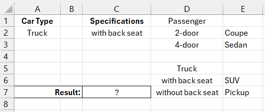
Cells A2 and C2 contain drop-down lists. Car features are listed in two ranges of cells below these tables, D2:D3 and D6:D7. Create drop-down lists by selecting: "DATA" → "Data Tools" → "Data Validation." In the "Data Validation" window, set "Allow: List" and fill in the parameters as shown below:
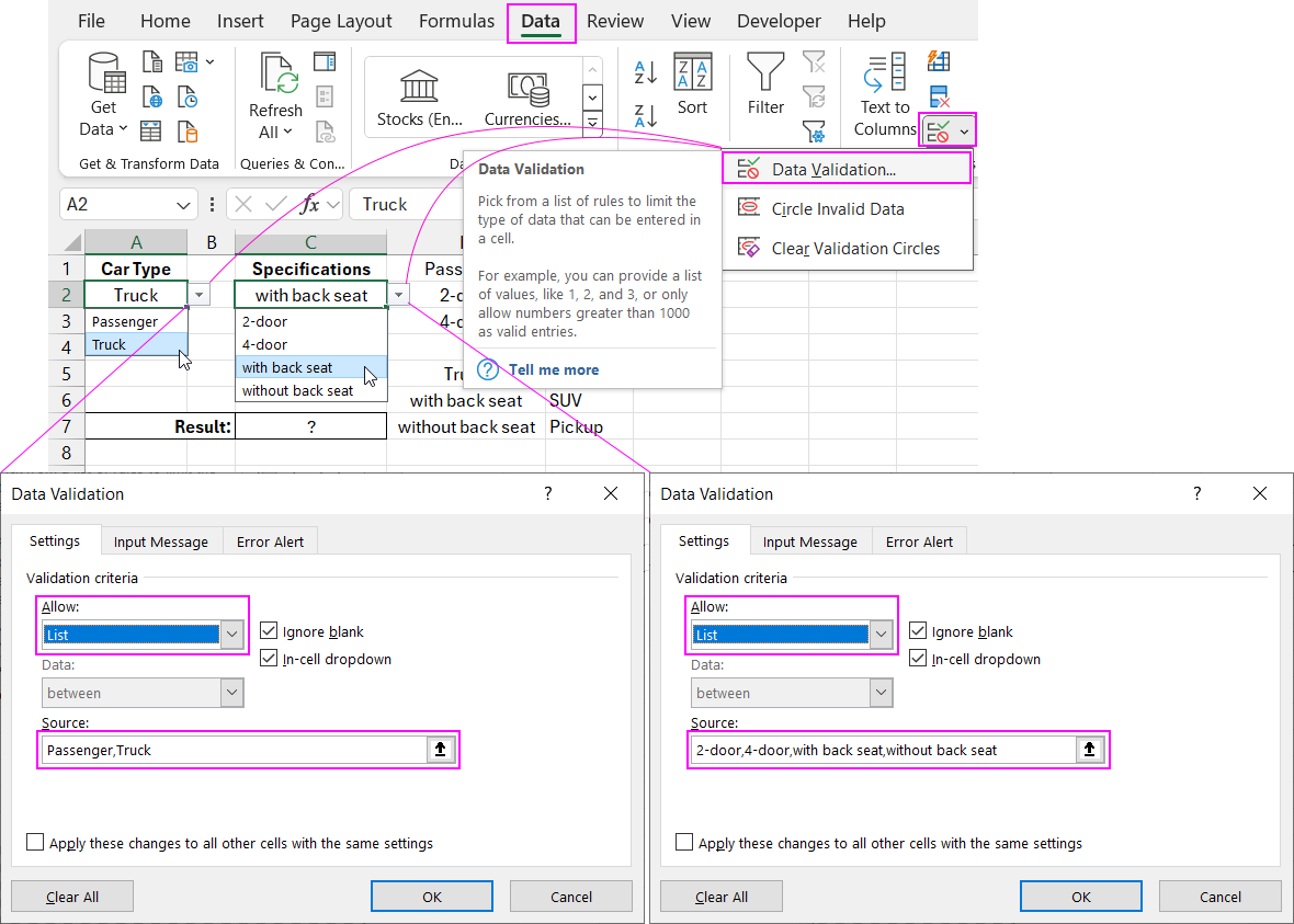
In this example, the formula in cell C7 returns the car body type: Sedan, Coupe, Pickup, or SUV, based on the car type and features selected:
=IF(A2="Passenger",IF(C2="2-door","Coupe","Sedan"),IF(C2="with back seat","SUV","Pickup"))
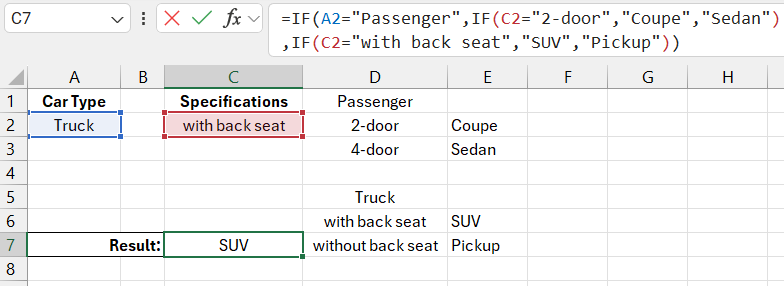
In this formula, the result of the first logical expression in the first condition affects the result returned by the second logical expression. See the figure:
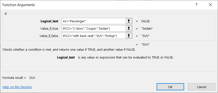
In this example, if the checked cell contains the value "Passenger Car," the second condition checks whether another cell contains "2-door" or "4-door." If the checked cell in the first condition contains "Truck," the second condition checks whether another cell contains "with rear seat" or "without rear seat."
The basic tool for performing conditional data analysis in Excel is the IF function. To analyze data with multiple conditions, you can nest IF functions. In the example above, the first IF function checks the content of cell A2. Instead of returning a result from the second argument, it calls a second IF function, which checks the value of cell C2 based on the second condition. Similarly, the third argument of the first IF function contains a third IF function, which checks the value of cell C2 based on another condition.
In the example image, the user selected the "Truck" car type from the drop-down list. The logical expression in the first IF function returned FALSE because the content of cell A2 was not equal to "Passenger Car." Therefore, the second argument of the first IF function is returned. This argument checked if cell C2 contained the value "with rear seat" and returned "SUV." If the user had selected "without rear seat" in the second drop-down list, the formula would have returned "Pickup" from the third argument of the third IF function.
Checking Multiple Conditions Without Using the IF Function
In older versions of Excel (before 2007), it was only possible to create up to seven levels of nested IF functions. Starting with Excel 2007, this limit was increased to 64 levels. As you can imagine, formulas with nested IF functions become difficult to read and use after about the fifth level, let alone with 7 or 64 levels. If you need more than 3-4 levels of nesting, it's worth looking for alternative methods.
Alternative Formula Using a Single IF Function and VLOOKUP
When a formula contains too many nested IF functions, it becomes hard to use and read. Below is a slightly different example of selecting a car body type. Instead of inputting constant values in the arguments of the IF function, you can refer to cells that contain the corresponding values. For example, next to the cell with the text "4-door," there is the text "Sedan." You can reference these values directly in the formula.
The new alternative formula would look like this:
=IF(A2=D1,VLOOKUP(C2,D2:E3,2,0),VLOOKUP(C2,D6:E7,2,0))

We got a similar result. The condition of the first IF function remains the same. However, the second argument now contains the VLOOKUP function, which can search for values based on the condition in the range D2:E3. In the third argument of the IF function, the VLOOKUP formula looks for values based on the condition in the range D6:E7.
Data Input Validation with Dynamic Drop-Down Lists
Drop-down lists for user input are shown in the example illustration of this article. This is a standard Excel data validation tool. The user does not input values into the cell but selects from a drop-down list.
Let's create a dependent drop-down list with dynamic value changes. You need to adjust the data validation rules for the drop-down list in cell C2 using an interesting technique with the function =INDIRECT(). Thanks to this function, the content of the drop-down list will change depending on the value in cell A2.
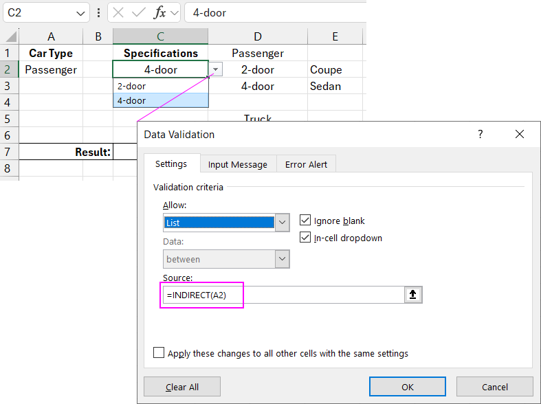
The image above shows the "Data Validation" window with the formula for the list in cell C2.
We also define names for cell ranges on sheet 2. The range named "Car" covers cells D2:D3, and the range named "Truck" refers to cells D6:D7. You can simply select the range and type the name in the "Name" field. Or create names by following the instructions: "FORMULAS"-"Name Manager"-"Create" as shown in the image below:
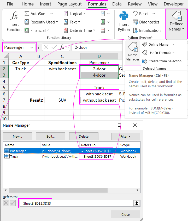
These range names exactly match the values of the first drop-down list in cell A2. And as you recall, the "Source" field contains the INDIRECT function with a reference to cell A2 in its argument.
The argument of the INDIRECT function gets text through the reference to cell A2. For example, in this case, the formula looks like: =INDIRECT("Truck") since cell A2 currently contains this text. This is also the name of the range. As a result of the calculations, the INDIRECT function returns a reference to the range D6:D7. The values from these cells are used for the second drop-down list in cell C2. When cell A2 contains the word "Car," the INDIRECT function returns a reference to the other range D2:D3, which would be used for the second drop-down list. Thus, we get a dynamic drop-down list in cell C2, which changes its values based on the first drop-down list selection.
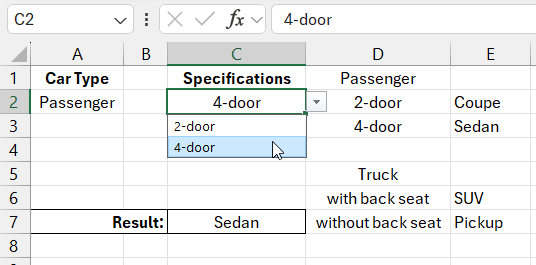
Now the linked drop-down list contains no unnecessary options, as it should.
The only problem with this example is that when the user changes the value in cell A2, the value in C2 doesn’t automatically update. The list of values updates, but the cell’s value will update only after using the drop-down. Therefore, the user must use both lists to refresh the values in both cells. Otherwise, incorrect formula results may occur.
Macro for Linked Dynamic Drop-Down List
However, we can write a simple macro for our sheet to clear cell B2 each time the drop-down list in A2 is used. To do this, open the VBA macro editor: "DEVELOPER"-"Visual Basic" or press ALT+F11. Then, insert this code into the sheet where the table is located:
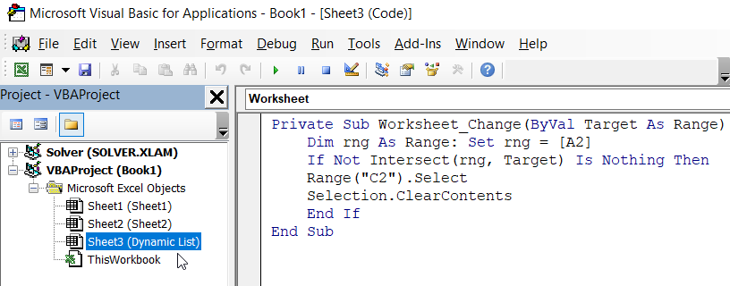
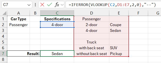
And in cell C7, where the old formula was, we enter the new formula with the VLOOKUP function:
=IFERROR(VLOOKUP(C2,D1:E7,2,0),"--")
Download examples of value validation with multiple conditions in Excel 
As a result, we don’t need the IF function for validating values based on multiple conditions.
Everything should be simple and elegant, as that's the magic!
