How to Use INDEX and MATCH to Retrieve Data in Excel
It often happens that when reading column values from tables, the lookup should be performed using the rightmost columns. Excel offers several functions that return cell values from the left side of the column being searched.
How to Apply the INDEX and MATCH Formula in Excel
Below is a picture of cities and regions where the network's stores are located. Suppose after the user selects a region from the dropdown list in cell G1, the fields "City" in G2 and "Store Number" in G3 should be automatically filled:
=INDEX(A2:D11,MATCH(G1,C2:C11,0),1)
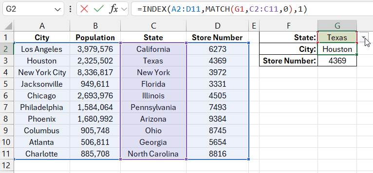
The INDEX function returns the value of a cell located in a specific row and column of a given range. In this case, the function’s range argument refers to the original store table. The second argument specifies the row number, and the third—the column number. In the formula for finding the city, the values are read from the first column, so the last argument contains the number 1.
The formula for finding the store number by the city name returns values from the fourth column:
=INDEX(A2:D11,MATCH(G1,C2:C11,0),4)
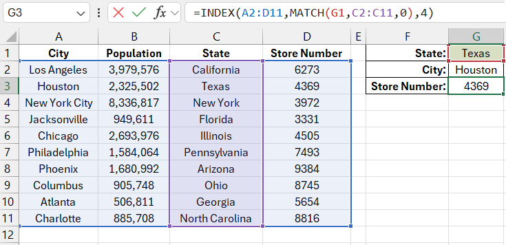
So, the last argument in the MATCH function equals 4.
If the cell range does not start at cell A1, the arguments defining the row and column do not correspond to the row and column numbers of the Excel worksheet. The numbering starts from the top-left cell of the specified range (in this example, A2) in the first argument of the INDEX function. For instance, the formula =INDEX(G2:P10,2,2) returns the value of cell H3, which is in the second row and second column of the G2:P10 range.
The second argument of the INDEX function contains the MATCH function. Its arguments always refer to a range of cells containing only one row or one column. If a range with more than one row or column is specified, the MATCH function returns the #N/A! error.
To get the correct row number for the INDEX function, you need to use the MATCH function, which returns the position of the found value in the table. The MATCH function uses three arguments in its syntax:
- Lookup value – what needs to be found.
- Lookup array – a one-dimensional array or range of cells from a single row or column where the value should be found.
- Match type – the exact match option (optional argument), with FALSE or 0 for an exact match. If an approximate match is required, use TRUE or 1.
In this example, the lookup value is the region name entered in cell G1. The formula searches for this value in the region list in the range C2:C11. The MATCH function sequentially checks all the cells until it finds the row "Sverdlovsk," which is in the 5th position. The function then returns the value 5, which is used as the second argument (row number) for the INDEX function.
After returning the result through the MATCH function, the INDEX function will have all the necessary data to display the corresponding value. It will move to the 5th row of the range and select the value from the first column "City" or from the fourth column "Store Number."
Note! If you specify a row number greater than the number of rows in the cell range or a column number greater than the number of columns, the INDEX function will return the #REF! error.
How to Lookup Values Using the LOOKUP Formula in Excel
A formula combining the INDEX and MATCH functions is the most popular formula type for looking up values in an Excel table. The LOOKUP function is used much less frequently. It uses three arguments in its syntax:
- Lookup value – the value whose position needs to be found.
- Lookup vector – a one-dimensional array or range of cells from a single row or column where the value is searched.
- Result vector – a one-dimensional array or range of cells from a single row or column from which the result should be returned (optional).
Note! The LOOKUP function has significant limitations:
- It cannot perform an exact match like the VLOOKUP, HLOOKUP, and MATCH functions.
- The lookup vector must be sorted in ascending order, otherwise, the function will return incorrect results, as shown in the image:
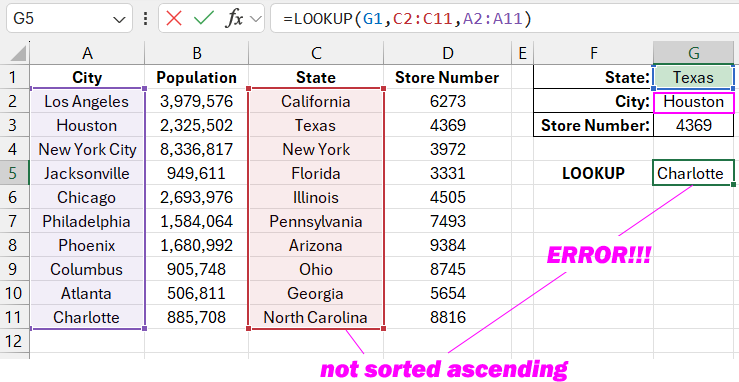
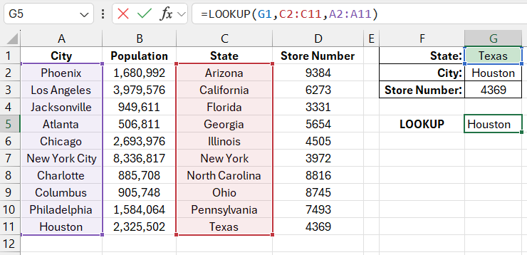
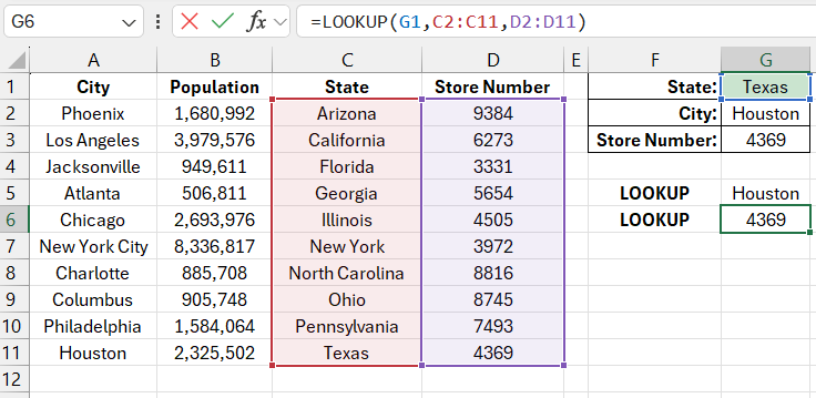
Therefore, before applying the function, sort the lookup vector in ascending order. The following two formulas are designed for an alternative city lookup:
=LOOKUP(G1,C2:C11,A2:A11)
And the corresponding store number:
=LOOKUP(G1,C2:C11,D2:D11)
Download Examples of INDEX and MATCH Formulas for Extracting Data in Excel 
The table has been sorted by the C2:C11 range in ascending order, and now everything works as expected.
The first two arguments of the LOOKUP function are the same as in the MATCH function. Both functions operate on the same principle, searching for a given value in one direction of the vector. The difference is that LOOKUP does not return the position of the found cell but the content of the corresponding cell in the result vector. Remember, the LOOKUP function requires sorting the table in ascending order and does not offer an exact match option when searching for values.
To find the desired city, the LOOKUP function first determines that the row "Sverdlovsk" is in the 10th position (after sorting the table) in the lookup vector range C2:C11. The formula then returns the content of the 10th cell, but from the result vector in the range A2:A11. The same principle applies when searching for the store number, but the result vector is in the D2:D11 range.
