How to Use SUMIF Formula to Get Values by Condition in Excel

Simple logical functions like IF are usually designed to work with a single column or a single cell. Excel also offers several other logical functions that are used to aggregate data. For example, the SUMIF function for selectively summing a range of values based on a condition.

Examples of a Sum Formula for Ranges with a Condition in Excel

The image below shows a table with a list of accounts, along with their status as positive or negative numbers. Let's say we need to calculate the sum of all negative numbers to determine the total expenditure of financial transactions. This result will later be compared with the sum of positive numbers to verify and determine the balance. We'll find out whether the income and expenses match – whether the debit equals the credit. To sum numerical values based on a condition in Excel, the SUMIF logical function is used:

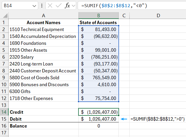
The SUMIF function analyzes each cell value in the range B2:B12 and checks whether it meets the specified condition (indicated in the second argument of the function). If the value is less than 0, the condition is met, and that number is included in the total sum. Values greater than or equal to zero are ignored by the function. Text values and empty cells are also ignored.

In the given example, the value in cell B2 is checked first, and since it is greater than 0, it is ignored. Then, cell B3 is checked, and since the numerical value is less than zero, the condition is met, so it is added to the total sum. This process is repeated for each cell. As a result, the values in cells B3, B6, B7, B8, and B10 are summed, while the other cells are excluded from the final sum.

Note that below the result of summing the negative numbers, there is a formula for summing the positive numbers. The only difference between them is the reverse comparison operator in the second argument where the condition for summing is specified – instead of "<0" (less than zero), ">0" (greater than zero) is used. Now we can verify that the debit equals the credit, and the balance will be zero if we add them together in cell B16 using the formula =B15+B14.

Example of a Logical Expression in a Sum Formula with a Condition

Another example is when we need to separately sum prices for product groups costing up to 1000 and those costing more than 1000. In this case, one comparison operator (<1000) is not enough, so we use the "less than or equal to" operator (<=1000); otherwise, prices exactly equal to 1000 would not be included in the calculation. Moreover, in this case, we cannot use "greater than or equal to" (>=1000) in the other formula, or we will sum the value of exactly 1000 twice, leading to incorrect final results:

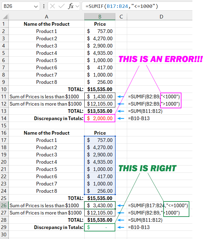
This is a very common mistake made by Excel users when working with logical functions!

Attention! In the first example, we did not need to account for zero values because they would not have affected the balance, but in the second case, the sum condition must be carefully defined to avoid calculation errors.

The second argument of the SUMIF function, i.e., the condition that must be met, is written within double quotes. In this example, a comparison symbol – "less than" (<) is used. By the function's syntax, such entries must be represented as a string, meaning within double quotes. Otherwise, Excel will issue a formula error warning.

Syntax of the Sum Formula with a Condition in Excel

The syntax of the SUMIF function includes an optional third argument – the sum range. In the previous example, the condition was checked against the same range that needed to be summed. Thanks to the third argument, it is possible to check conditions in one range and sum values in another.

The image below shows a sales report table by customers for the month. Next to each customer is the amount spent on purchases throughout the month. Some customers made multiple purchases during the month, so their names are duplicated in the list. We need to find out the total amount spent by "Customer3" during this month. Here, it's appropriate to use a formula with the third argument of the SUMIF function filled in:

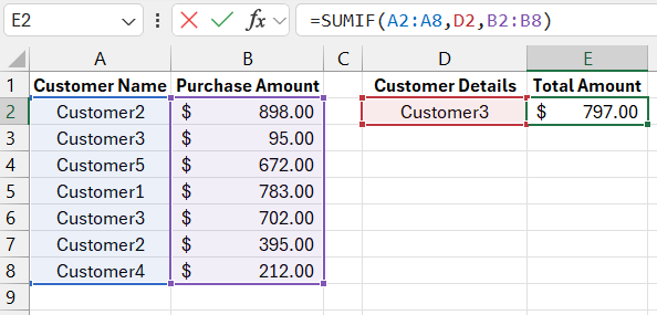
As seen in all the above examples, the second argument specifies a string of text with the condition, not a logical expression like in the IF function. In practice, this second logical argument with the condition in the SUMIF function can contain:

strings with text values;
numerical values;
logical expressions;
formulas with functions;
cell references.

Next, we will look at more examples of creating conditions for the second logical argument of the SUMIF function in more detail.

Creating Condition Criteria for the SUMIF Function

The second argument of the function is called the "Criteria." This logical argument is also used in other similar logical functions: SUMIFS, COUNTIF, COUNTIFS, AVERAGEIF, and AVERAGEIFS. In all cases, the argument is filled in according to the same rules for creating logical conditions. In other words, for all these functions, the second argument with the condition criteria is a logical expression that returns either TRUE or FALSE. This means that the expression must contain a comparison operator, such as: greater than (>), less than (<), equal to (=), not equal to (<>), greater than or equal to (>=), or less than or equal to (<=). You can omit the equal sign (=) if you're checking for an exact match.

Creating complex condition criteria can be confusing. However, if you follow a few simple rules, as described in the table below, you won’t encounter any issues.

Table of Rules for Creating Condition Criteria:

To create a condition	Follow this rule	Example
The value equals a specific number or the address of a cell.	Do not use the equal sign or double quotes.	=SUMIF(B1:B10,3)
The value equals a text string.	Do not use the equal sign, but use double quotes around the text.	=SUMIF(B1:B10,"Client5")
The value differs from a specific number.	Place the operator and the number in double quotes.	=SUMIF(B1:B10,">=50")
The value differs from a text string.	Place the operator and the text in double quotes.	=SUMIF(B1:B10,"<>payment")
The value differs from the content of a referenced cell or the result of a formula.	Place the comparison operator in double quotes and connect it with an ampersand (&) to the cell reference or formula.	=SUMIF(A1:A10,"<"&C1) or =SUMIF(B1:B10,"<>"&TODAY())
The value contains a portion of a string.	Use wildcard operators and enclose them in double quotes.	=SUMIF(A1:A10,"kg";B1:B10)

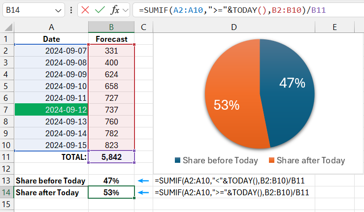
In the second argument for condition criteria, you can use various functions and formulas. The image below shows a list of dates and their assigned values. It is important to note that today’s date at the time of writing is "03.11.2018." To sum numerical values only for today's date, use the formula:

=SUMIF(A2:A10,"<"&TODAY(),B2:B10)/B11

To sum only values from today onward until the end of the period, use the "greater than or equal to" (>=) operator together with the corresponding function =TODAY(). The formula with the operator (>=):

=SUMIF(A2:A10,">="&TODAY(),B2:B10)/B11

Summing Based on Partial Matches in Condition Criteria

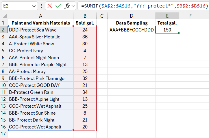
In the second logical argument for condition criteria in the SUMIF function, you can apply wildcard characters (?) and (*) to create relative, imprecise queries. The question mark (?) represents any single character, while the asterisk (*) stands for any number of characters or an empty string. For example, if you need to sum only protective paints with a code consisting of 3 English letters at the beginning of the name:

=SUMIF($A$2:$A$16,"???-protect*",$B$2:$B$16)

Download an example of how to use the SUMIF formula to filter values in Excel download file

All values in the range B2:B16 are summed according to the values in the A2:A16 range, where the string fragment "-protection" follows the third character.

This way, we successfully summed only a specific group of products from the general warehouse report list. The product name fragment must appear in a specific place – 3 characters from the start of the string. There is no need to use complex formulas like =LEFT() and so on. You can simply use wildcard operators to create a simple and concise query to the database with minimal system resource usage.