How to use SUMIFS formula in Excel with multiple conditions
The SUMIF function in Excel is designed for summing values based on a condition. Its main drawback is that it allows only one criterion for the condition. If there is a need to use multiple conditions, you can use the SUMIFS function, which is available in newer versions of Excel starting from 2010.
SUMIFS function for summing values with multiple conditions
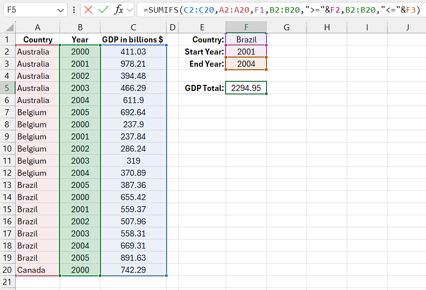
Below is a portion of a list of countries with GDP figures for the period from the 2000s to 2005. Suppose we need to sum Brazil's GDP for 2001-2004. To sum values based on two or more conditions, it is convenient to use the SUMIFS function. In this case, we need to consider:
- The first condition – only the country Brazil.
- The second condition – sum GDP only for 2001 and 2004.
The formula for calculating the sum of GDP indicators for the specified country over a specific period of years:
=SUMIFS(C2:C20,A2:A20,F1,B2:B20,">="&F2,B2:B20,"<="&F3)

The first argument of the SUMIFS function is the range of cells containing the values to sum. The following arguments are grouped in pairs following the pattern Criteria_Range1 together with Criteria1. The number of arguments in the function is always an odd number, considering their sequence. The first pair of criteria (the second and third arguments) are mandatory. Without them, this function would be no different from the regular SUM function. Additional subsequent pairs of criteria are optional. The maximum number of argument pairs can reach up to 127. That is, the maximum number of all arguments in the SUMIFS function is 127*2+1=255.
In the example above, the values in column C are summed only for those cells that meet the conditions in columns A and B. The condition for selecting cells in column A is matching the value in cell F1, where the country name is specified for selection. The year is checked against two conditions defining the starting year and the end period. The starting year is recorded in cell F2, and the end year in F3. References to these cells, combined with the comparison operators "greater than or equal to" (>=) and "less than or equal to" (<=), ensure that the value of the cell in column D will only be included in the total if all three conditions are met.
Alternative SUMPRODUCT function for summing with multiple conditions
The SUMIFS function appeared only in relatively new versions of Excel in 2010. In older versions, the best way to sum values with two or more conditions was to use the SUMPRODUCT function. It contains only one required argument but offers expanded capabilities. In this example, the task can be solved using another formula:
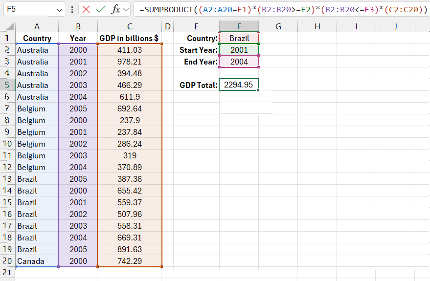
=SUMPRODUCT((A2:A20=F1)*(B2:B20>=F2)*(B2:B20<=F3)*(C2:C20))

As shown in the figure, this SUMPRODUCT formula in its first argument contains pairs of cell ranges and logical expressions with conditions, similar to the previous function. Within each pair of parentheses (except the last one) are ranges of cells and comparison operators with values. The last pair of parentheses simply contains the address of the overall range of filled cells in column D.
Excel interprets each logical expression in this formula as a separate table of values.
Fun fact! The sequence of expressions in parentheses of this formula is not mandatory, unlike the required sequence of arguments in the previous SUMIFS function. For example, the summing range can be in the first pair of parentheses or in any other place, and this will not affect the result of the calculation.
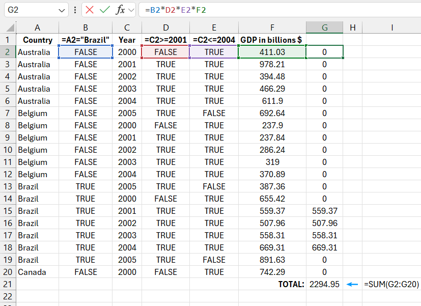
The principle of the SUMPRODUCT function is based on table arrays. These are tables created in memory that represent lists of values. In the SUMPRODUCT function, each element of the table is compared with its corresponding value. For example, in the above example, each cell in the range A2:A20 is first checked against the value in F1. The function looks for the addresses of cells that contain the value "Brazil". The result of these comparisons is a new table containing a list of TRUE and FALSE values, corresponding to each cell of the original table. These resulting logical values in memory are called elements. Most of them will naturally be false elements (in this example), but 6 elements correspond to cells containing the string "Brazil" and are given the TRUE value.
Four pairs of parentheses correspond to four tables that are multiplied together. Essentially, each element of each table is multiplied by the current element of every other table. In Excel, the logical value TRUE = 1, and FALSE = 0. As a result, if even one of the 4 multiplying current elements returns a value of 0, the resulting current element also returns a value of 0 – meaning FALSE. After all, any number multiplied by zero equals 0. However, if each current multiplying element has the value TRUE, the element in the resulting table will have the current cell value in the range D2:D20, as the three ones will be multiplied together with the current value from column D.
This process can be described schematically. On the fourth row of the sheet, i.e., the third row of the table section, we have data on Australia's GDP for 2002. When processing this row with the SUMPRODUCT function, all values in the current cells are checked and multiplied together in memory as follows:
FALSE*TRUE*TRUE*394.48
In other words:
(the country name is not Brazil)*(the year is greater than 2001)*(the year is less than 2004)*(current GDP value)
Or like this:
0*1*1*394.48=0
The first zero is the result of checking the first table array, which returned a logical value of FALSE – not equal to Brazil! Since one of the multiplying numbers is zero, the result of simple arithmetic operations is also 0.
In the case of the 15th row of the sheet, a completely different situation arises. All the check results return TRUE, which means =1. This time, the first cell is found to contain the text "Brazil". When checking the year for "greater than or equal to" >=2001, we again get TRUE. This same cell with the year is now checked under the third condition "less than or equal to 2005" and again returns TRUE. Thus, the following operation is performed:
1*1*1*559.37=559.37
For clarity, here is a table:

Download examples of how to use summation formulas with multiple conditions in Excel 
This is the final result for the 15th row of the sheet, the 14th row of the table in memory. The same operations are performed for the other rows of the table. For each row, the final result (0 or the GDP figure) is calculated and summed using the SUMPRODUCT function. This function is quite complex and works slower than SUMIFS, but it can still be used in newer versions of Excel as experienced users are accustomed to it. This also allows older versions of files to be opened without errors in the formulas. In some rare cases, it may even be more convenient than other functions, so it’s worth understanding its principles.
