How to Use SUMPRODUCT Formula for Multiple Criteria in Excel

To search for values based on multiple criteria, the SUMPRODUCT function is highly effective. This function is supported in all versions of Excel. When used in formulas along with other functions, SUMPRODUCT allows searching not only for numbers but also for text.

How the SUMPRODUCT Function Works with Multiple Criteria

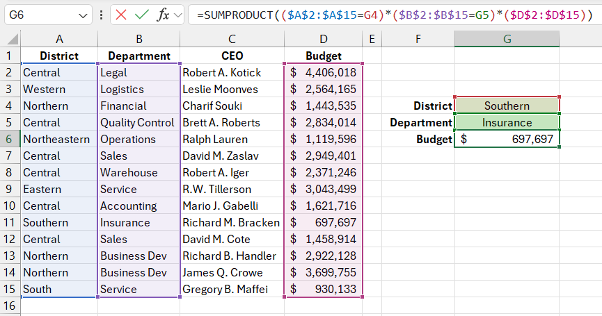
Below is an image of a table showing departments and their budgets. Suppose we need to create a formula that, after selecting two criteria from the user: region and department, will return the corresponding budget amount. In this case, you can't simply use VLOOKUP as it only searches for one value based on a single criterion. In this example, you need to find two criteria simultaneously, as region and department names are repeated multiple times in the source table.

To obtain a value from a row that matches both criteria, you can use the following formula:

=SUMPRODUCT(($A$2:$A$15=G4)*($B$2:$B$15=G5)*($D$2:$D$15))

The SUMPRODUCT function works by checking each cell's value in specified ranges A2:A15 and B2:B15 against the criteria in cells G4 and G5. The result of the comparisons returns arrays of TRUE or FALSE values. When multiplied together in the formula, TRUE is treated as 1 and FALSE as 0. The range in the third pair of parentheses in the first argument of the SUMPRODUCT function contains the final values, one of which is correct and will be returned by the function.

If the result of comparing cells in the "Region" or "Department" columns returns FALSE, then the calculated sum for that row will be zero (0), because FALSE is replaced by 0. If the region and department names match, the result of both comparisons will be 1. These ones will be multiplied together, resulting in 1, which will then be multiplied by the numeric value in the "Budget" column, giving the final result.

In the example shown, the SUMPRODUCT function reads data from row 11 and performs the arithmetic operation 1*1*697,697 = 697,697. This number is then summed with the results of multiplications in other rows, which are all 0. This is because multiplying by even one zero (from the FALSE value) results in 0, as seen in the last row of the table: 1*0*930,133 = 0.

Finding Text with the SUMPRODUCT Function with Multiple Criteria in Excel

The SUMPRODUCT function can only be used in the described manner when the return value is a number. If the result should be text, then all text strings would be counted as zeros, and the function would constantly return a final value of 0.

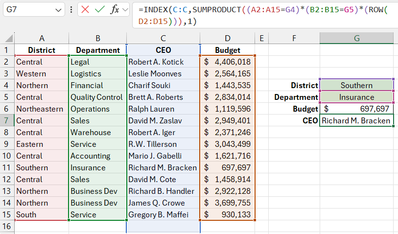
However, you can combine the SUMPRODUCT function with the INDEX and ROW functions in one formula. This allows the result to be returned as text. For example, to return the name and surname of a department head, you can use the following formula:

=INDEX(C:C,SUMPRODUCT((A2:A15=G4)*(B2:B15=G5)*(ROW(D2:D15))),1)

Finding text with the SUMPRODUCT function.

Download example of using SUMPRODUCT formula with multiple criteria in Excel download file

In this formula, instead of cell ranges from column D, the ROW function is used to return the number for each current row of the source table. The SUMPRODUCT function analyzes the Excel sheet's row number 11 and performs the multiplication operation: 1*1*12 = 12. This multiplication result is then used as an argument for the INDEX function, which covers the entire column C:C, since the ROW function returns row numbers of the Excel worksheet, not the source table.