How to Use VLOOKUP in Excel to Search Across Two Tables
Sometimes the data you need to find may be located in different tables. It is often necessary to extract data from multiple Excel tables. The user should be able to determine which table to pull data from based on criteria for different data types. A special formula can be created for this purpose.
How to Link Two Tables with One VLOOKUP Formula Based on a Condition
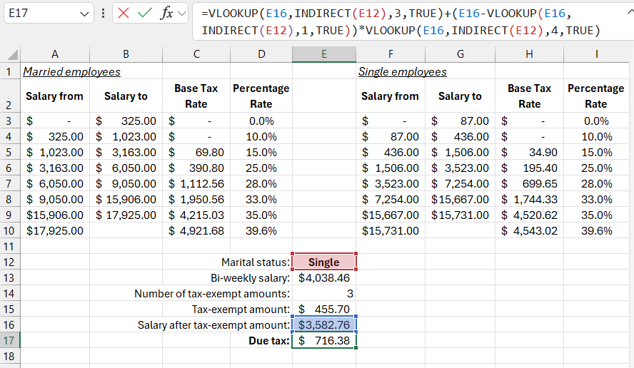
Below is an image of a table used to calculate tax amounts. The user has the option to determine an employee's marital status (Married or Unmarried). If the user selects the "Unmarried" condition, the data will be extracted from the "Unmarried Employees" table. If "Married" is selected, the lookup will be done in the "Married Employees" table. The formula for calculating taxes based on whether the employee is married or unmarried:
=VLOOKUP(E16,INDIRECT(E12),3,TRUE)+(E16-VLOOKUP(E16,INDIRECT(E12),1,TRUE))*VLOOKUP(E16,INDIRECT(E12),4,TRUE)

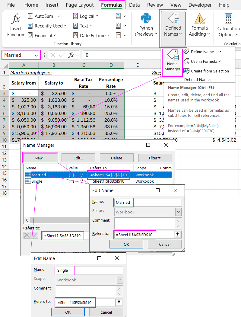
To create a switch between tables, you can use named cell ranges and the INDIRECT function. Then, you need to create the formula. First, create two named ranges:
- Married – for the "Married Employees" table.
- Unmarried – for the "Unmarried Employees" table.
To assign unique names to the ranges from these two tables, follow these steps:
- Select the range of cells A3:D10.
- Select the tool: "FORMULAS" – "Defined Names" – "Define Name." The "New Name" window will appear as shown in the image:
- In the "Name:" field, enter "Married" and click OK.
- Select the range of cells from the second table F3:I10.
- Again, select the "Define Name" tool from the "FORMULAS" tab and fill in the "Name:" field with "Unmarried."
- Click OK.

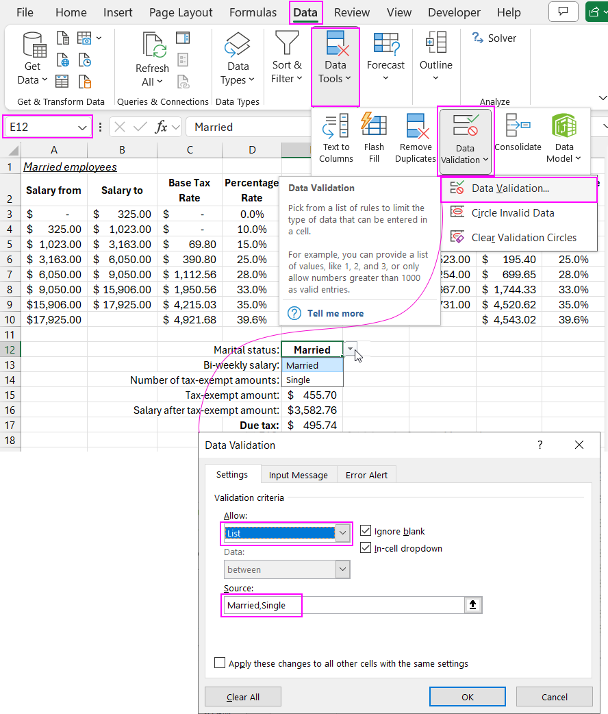
For precise and convenient input of values, a dropdown list is used in the cell, created with the tool: "DATA" – "Data Tools" – "Data Validation" – "Allow:" – "List."

Download the VLOOKUP formula example for merging two tables in Excel 
The dropdown list contains only two values: "Married" and "Unmarried," exactly matching the names of the named cell ranges created earlier. The value in cell E12 will be used to switch between tables based on the condition. Therefore, the values and named ranges must be identical.
The core of this formula is the VLOOKUP function. Its second argument, which specifies the source table, contains the INDIRECT function. This function has the first argument "Ref_text," which converts the incoming text into a cell or range reference. In the first image, cell E12 contains the value "Unmarried." The INDIRECT function tries to convert this text into a cell or named range reference. If the text cannot be converted into a cell reference (as in this example), the INDIRECT function checks whether there are any named ranges with that name in the workbook. If such named ranges were not created, the function would return a #REF! error.
The INDIRECT function's syntax includes a second optional argument called "A1." A TRUE value in this argument means the reference is in A1 notation, and a FALSE value means it's in R1C1 notation. In the case of named ranges, the INDIRECT function will return the correct result regardless of whether the second optional argument "A1" is set to TRUE or FALSE.
The INDIRECT function can also return external references to other sheets or even other Excel workbooks, provided that the workbook being referenced is open. Otherwise, the function will return a #REF! error.
