INDIRECT Function in Excel formulas: Usage with Examples
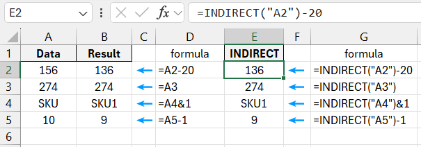
The INDIRECT function returns a reference specified by a text string. For example, the formula =INDIRECT(A3) is similar to the formula =A3. However, in INDIRECT, the reference is treated as a text string, allowing it to be dynamically modified using formulas.
The function is used for adjusting cell references without altering the formula, extracting values from odd/even rows, transposing tables, and more.
Syntax of the INDIRECT Function with Explanation
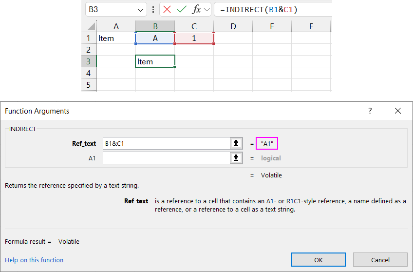
=INDIRECT(B1&C1,TRUE)
Arguments:
- Text reference: A mandatory argument containing the cell reference as a text string. For instance, =INDIRECT("A1") or =INDIRECT("Sheet2!A3").
- A1: An optional logical argument that defines the reference type. If TRUE (or omitted), the text is treated as an A1-style reference (explicit cell address). If FALSE, it is treated as an R1C1-style reference (relative to the formula's position).
Why Errors Occur with INDIRECT Function
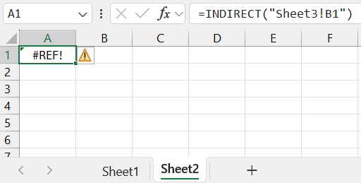
- The "text reference" argument specifies an invalid reference, resulting in a #REF! error.
- The argument points to another workbook (an external reference) that is inaccessible or closed, causing a #REF! error. External data sources must remain open when using such formulas.
- The argument specifies a range that exceeds the maximum limit—#REF! error. The function supports up to 1,048,576 rows or 16,384 columns.
Examples and Applications of the INDIRECT Function in Excel
Let’s begin with a simple example to understand how the function works.
Given the following data table:
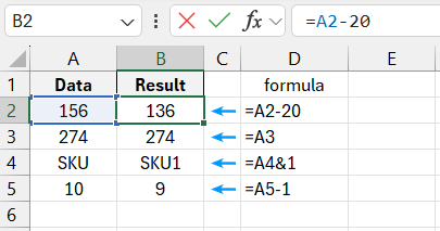
Examples of using the INDIRECT function:
Consider this practical scenario: On worksheets named 2025, 2026, 2027, 2028, 2029, and 2030, identical data is stored in the same cells (e.g., employee education information for the last 5 years).
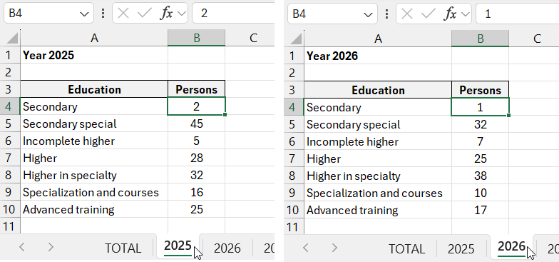
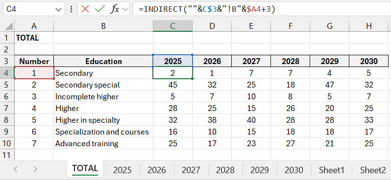
We aim to compile the data from these sheets into a consolidated table on a separate worksheet. Here's how to achieve this using the INDIRECT function:
Enter the formula in cell B4 and copy it across the range B4:H10 to populate the consolidated table with data from the five worksheets.
=INDIRECT(""&C$3&"!B"&$A4+3)
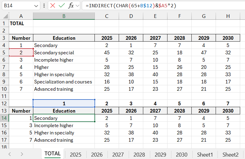
Now, extract values from only the odd-numbered rows in the consolidated table. For convenience, label columns and rows:
To retrieve entries from odd rows, use this formula:
=INDIRECT(CHAR(65+B$12)&$A5*2)
For extracting values from even-numbered rows:
=INDIRECT(CHAR(65+B$19)&$A5*2+1)
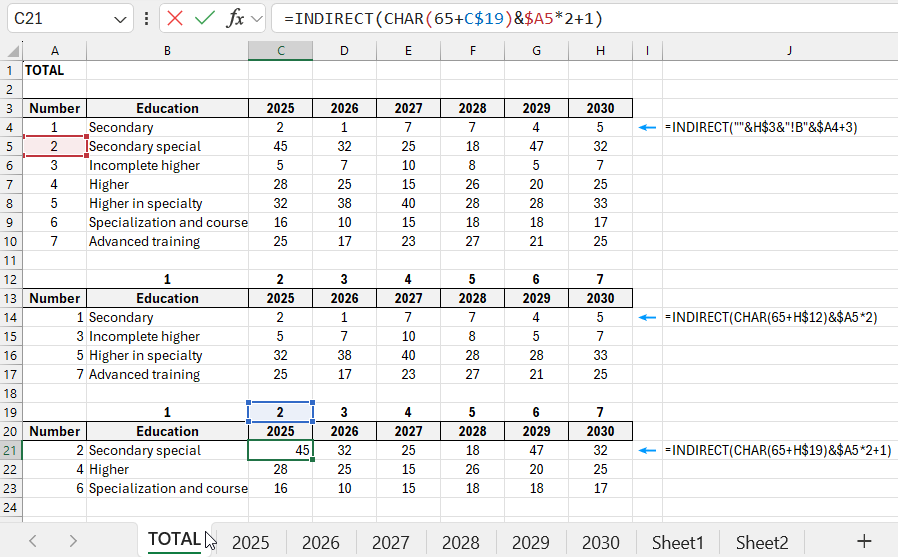 Note: The CHAR function returns a character based on the specified code. Code 65 outputs the letter 'A,' 66 = 'B,' 67 = 'C,' and so forth.
How to Use the INDIRECT Function with VLOOKUP
Suppose the user has multiple data sources (in our example - several reports). We need to output the number of employees based on two criteria: "Year" and "Education". The VLOOKUP function is suitable for finding a specific value in a database.
To make the function work, place all the reports on one sheet.
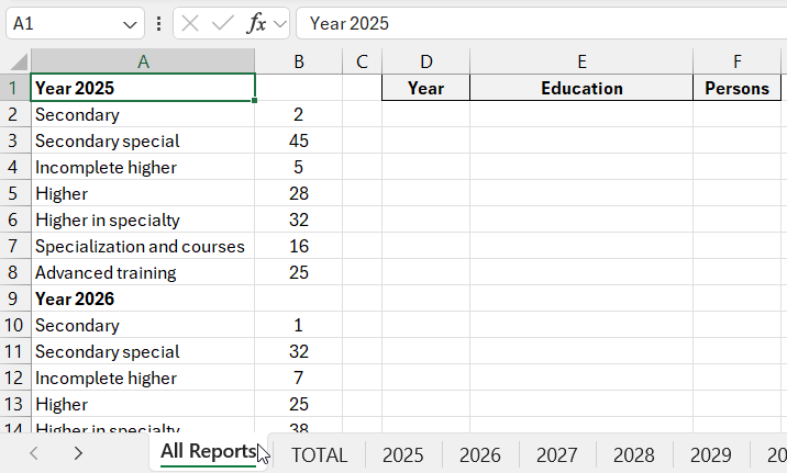
But the VLOOKUP function cannot process information in this form. Therefore, we gave each range of report cells a name (created named ranges). Separately, we made dropdown lists: "Year", "Education". The "Year" list contains the names of all the named ranges (Year_2025, Year_2026, Year_2027, Year_2028, Year_2029, Year_2030).
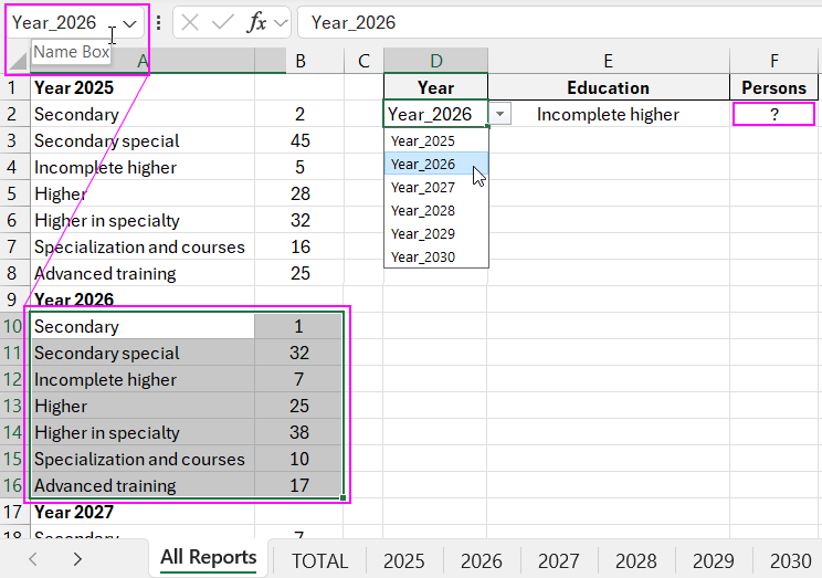
The task: When selecting the year and education, the number of employees should appear in the "Count" column.
If we only use the VLOOKUP function, a #N/A error will occur. Such a formula cannot process named ranges from cell values, but only if the name is specified in the second argument of the VLOOKUP function:
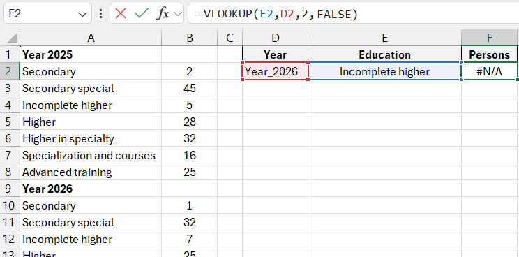
The formula does not perceive the D2 reference as a reference to the named range where the report for a particular year is located. Excel considers the value in cell D1 as plain text.
=VLOOKUP(E2,INDIRECT(D2),2,FALSE)
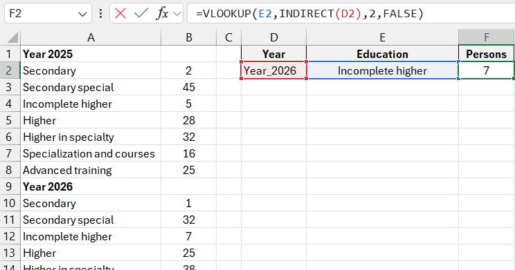
The INDIRECT function helped to fix the situation, which returns a reference to the named range specified by the text string in the value of cell D1.
Example of VLOOKUP and INDIRECT functions in Excel
Now the formula works correctly. To solve similar tasks, you need to use the VLOOKUP and INDIRECT functions in Excel simultaneously.
Suppose you need to extract information based on a given value. That is, achieve dynamic data substitution from different tables. For example, specify the number of employees with incomplete higher education in 2025 and 2026. Do the following:
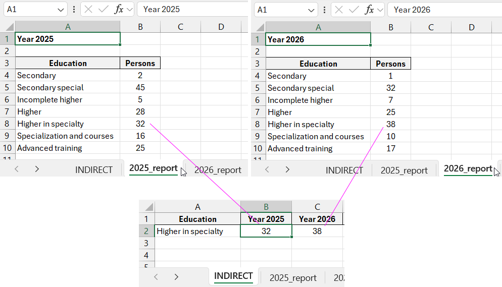
For two reports, the combination of VLOOKUP and IF functions works:

But for our five reports, using the IF function is impractical. To return the lookup range, it is better to use INDIRECT:
=VLOOKUP($A$2,INDIRECT(RIGHT(B1,4)&"_report!A3:B10"),2,FALSE)

- $A$12 – a reference with education (can be selected from a dropdown list);
- B1 – a cell that contains the first part of the sheet name, i.e., the year number. We extract it from the value of cell B1 using the RIGHT function to pass only the last 4 characters "2025" into the formula argument, not the full text "Year 2025". Then add the missing common text "_report!A3:B10" to create a reference to the cells with the report on different sheets (all sheets are renamed: "2025_report", "2026_report", etc.);
- "_report!A3:B10" – the common part of the names of all sheets and the report range. It is concatenated with the year value using the (&) operator. As a result, we get the full address of the desired range.
Download the example of formulas with INDIRECT function in Excel 
Thus, these two functions perform such tasks excellently.
