Using AND in IF Formula with Multiple Conditions in Excel
When validating cell values with multiple conditions, you don't have to rely solely on the IF function in formulas; you can use the logical function =AND(). This method works well in cases where you need to check two or more conditions simultaneously to determine the argument returned by the formula.
How to use the AND function for an IF formula with multiple conditions
Below in the image is a list of products, quantities, and the discounts applied during the sale. The code for each product consists of three parts, separated by dashes:
- The first part is the department number.
- The second part defines whether the item is an element (ELM), semi-finished product (PFB), or final product (FIN).
- The third part is a unique 4-character identifier.
Suppose we need to apply a 10% discount only to final products from department 202. No discounts are applied to other items. The formula is:
=IF(AND(LEFT(A2,3)="202",MID(A2,5,3)="FIN"),10%,0%)
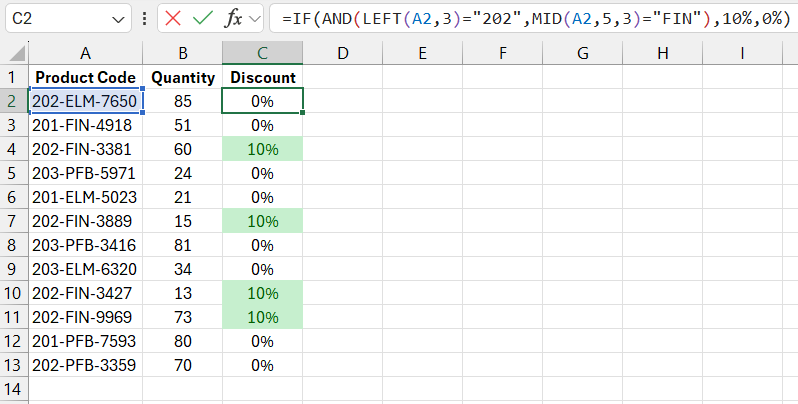
The IF function returns 10% only when the logical expression is TRUE; otherwise, it returns 0%. The first argument of the function should be a logical expression that returns TRUE if the first part of the product code equals 202. At the same time, the second part of the code should equal FIN.
Excel provides the =AND() function to implement this solution. This function can hold up to 255 logical arguments, separated by semicolons. Logical arguments are expressions that return either TRUE or FALSE. In the example above, the =AND() function contains only two logical arguments:
- The first logical expression: =LEFT(A2,3)="202" is used in the first argument and returns TRUE if the first three characters of the product code in cell A2 equal "202".
- The second logical expression: =MID(A2,5,3)="FIN" in the second argument returns TRUE if the three characters starting from the 5th character from the left equal "FIN".
For the =AND() function to return TRUE, all of its logical arguments must return TRUE. If any argument returns FALSE, the =AND() function will also return FALSE. This is easy to understand from the example in the table below, which shows the results returned by the =AND() function with two logical arguments:
| First logical argument | Second logical argument | AND function result |
| TRUE | TRUE | TRUE |
| TRUE | FALSE | FALSE |
| FALSE | TRUE | FALSE |
| FALSE | FALSE | FALSE |
In the formula in cell C2, the first logical argument of the =AND() function returns TRUE since the first three characters of the product code are equal to 202. However, the second argument returns FALSE because the middle part of the product code is ELM, not FIN. Based on the table above, the combination of TRUE and FALSE results in the =AND() function returning FALSE, and the entire formula returns 0%.
The =AND() function in the formula in cell C4 returns TRUE because both of its logical arguments returned TRUE.
Example of how the AND function works
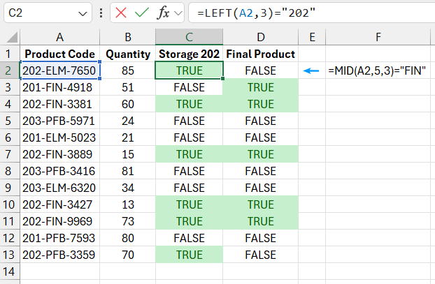
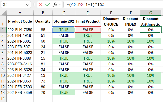
To visually demonstrate how the =AND() function and the formula as a whole work, let's look at another example for this same task. In the previous example, the =AND() function contains two arguments, each of which contains a logical expression that returns TRUE or FALSE. These arguments can also contain cell references instead of logical expressions. The important thing is that the referenced cells must contain logical values. To make things clearer, the product table now includes two additional columns, as shown in the image below. These columns allow users to analyze why certain products received or did not receive a discount:
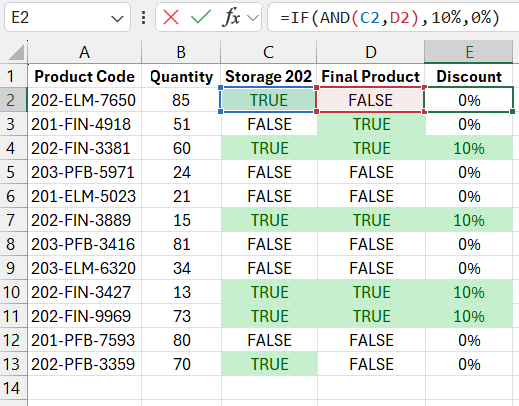
After modifying the table, we also simplified the formula:
=IF(AND(C2,D2),10%,0%)
Furthermore, we can simplify it even more, so that we don't even need the IF function when checking multiple conditions.
How to check a value against multiple conditions without using the IF function
What can replace the IF function in the formulas described above when analyzing multiple conditions in Excel? Considering the fact that logical values TRUE and FALSE can be represented by the numbers 1 and 0, respectively, you can perform mathematical operations on logical values in Excel. For example, TRUE+1=2 or FALSE-5=-5. Therefore, we can simplify the formula even further in several ways, such as replacing the IF function with CHOOSE or INDEX:
=CHOOSE(C2+D2+1,0%,0%,10%)
=INDEX({0,0,0.1},C2+D2+1)
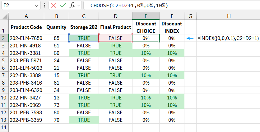
For this table, we can create a formula without using any functions, relying only on mathematical operations with logical values:
=(C2+D2-1=1)*10%
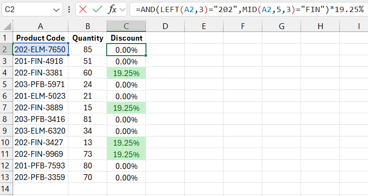
What is the key takeaway here? Thanks to the =AND() function in Excel, we can validate tables against multiple conditions without using the IF function to quickly create concise formulas. For a practical example, we can apply this knowledge to the first table and make the task more challenging by offering a 19.25% discount instead of 10%:
=AND(LEFT(A2,3)="202",MID(A2,5,3)="FIN")*19.25%
How to use AND function in IF Excel formula with multiple conditions
As you can see, we successfully validated the entire table against multiple conditions without using the IF function by replacing it with simple mathematical operations. However, it is worth noting that such a formula may be a bit harder to read.
