Using IFERROR and ISNA Formulas in Excel to Handle Errors
In Excel lookup functions like VLOOKUP, HLOOKUP, and MATCH, the value FALSE or 0 is often used in the third argument. This instructs Excel to search for exact matches in the source table. If the lookup function specifies an exact match in the third argument and the value is not found in the table, the function will return an #N/A! error.
IFERROR Formula for Handling VLOOKUP Errors in Excel
The #N/A! error can be useful when analyzing data models in Excel because it informs the user and the program that a matching value was not found. However, if much of this data model is used in reports, the #N/A! error code can look unprofessional. Excel offers functions that check for calculation errors and allow returning alternative values.
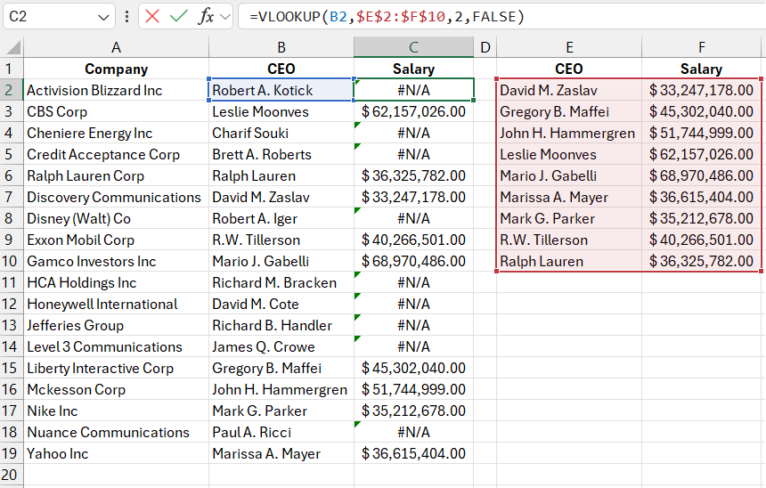
Below is an image of a table with company names and their executives. The second table contains the same last names and their corresponding salaries. The VLOOKUP function is used to merge the two tables into one. However, since salary data is not available for all executives, the #N/A! error code frequently appears in the VLOOKUP results.

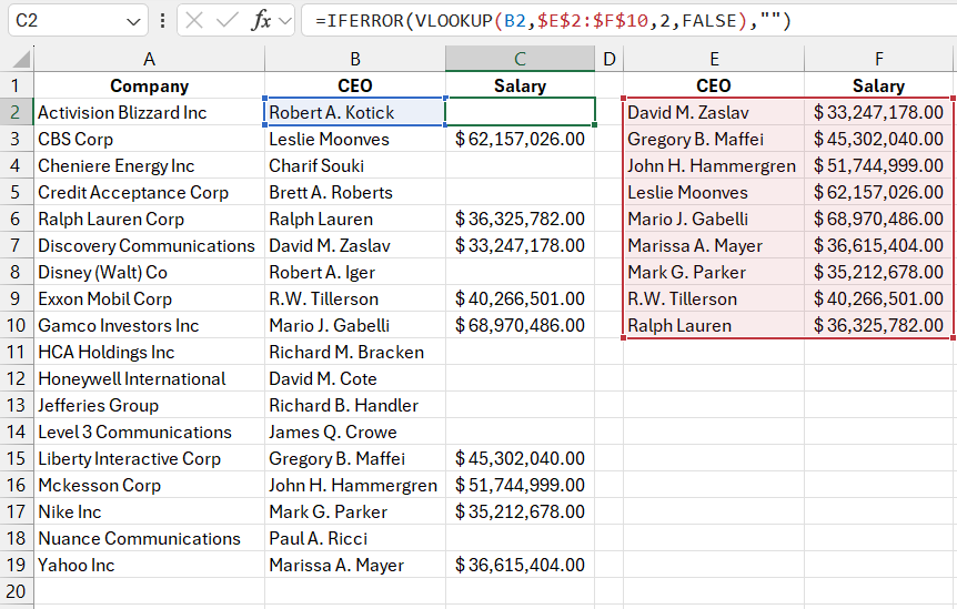
The formula shown in the next image has been modified to use the IFERROR function, which returns a blank string if the lookup value is not found in the source table:
=IFERROR(VLOOKUP(B2,$E$2:$F$10,2,FALSE),"")

Users often refer to this function as "error hiding" because it detects and conceals errors, making reports cleaner for presentation purposes.
The first argument of the IFERROR function is an expression or formula, and the second argument specifies the alternative value to display if an error occurs. If the first argument’s expression or formula returns an error, the function returns the second argument’s value instead. Otherwise, it returns the result of the first argument.
In this example, the alternative value is a blank string (two quotation marks with nothing between them). This improves the report’s readability and presentation. The function can also return other values, such as "No Data" or the number 0.
Functions for Handling Error Codes in Excel
The IFERROR function checks for any error a formula in Excel may return. However, it should be used cautiously, as it hides all errors, even critical ones like #DIV/0! or #VALUE!.
To hide only specific types of errors, Excel offers three other functions:
- ISERROR – Returns TRUE if its argument contains an error: #N/A, #VALUE!, #REF!, #DIV/0!, #NUM!, #NAME?, or #NULL.
- ISERR – Returns TRUE if its argument contains any error except #N/A!.
- ISNA – Returns TRUE if its argument contains an #N/A! error, or FALSE for any other value or error.
These three error-handling functions in Excel return logical values of TRUE or FALSE and are often used in combination with the IF function.
IF and ISNA Formula for VLOOKUP Errors Without IFERROR in Excel
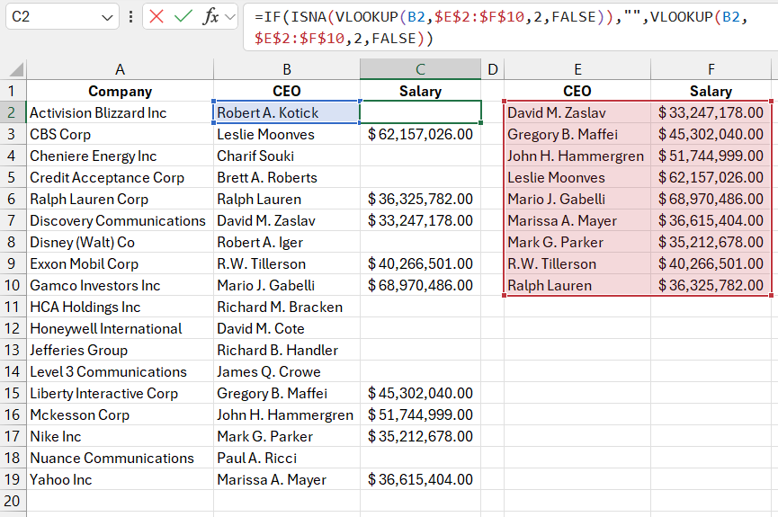
The robust IFERROR error-handling function was introduced in Excel starting with the 2010 version. In older versions of Excel, the ISNA function was most commonly used for error checking:
=IF(ISNA(VLOOKUP(B2,$E$2:$F$10,2,FALSE)),"",VLOOKUP(B2,$E$2:$F$10,2,FALSE))

Download Examples of IFERROR and ISNA Formulas for Error Handling in Excel 
The ISNA function returns a logical value of TRUE if its argument contains only one type of error—#N/A! Or FALSE for any other value. In this formula, the IF function works with ISNA. If the #N/A! error is detected, the formula returns a blank string, as indicated in the second argument of the IF function. Otherwise, it returns the VLOOKUP result, specified in the third argument of the IF function.
The main drawback of this formula is the need to duplicate the VLOOKUP function:
- First, inside the ISNA function;
- Second, in the third argument of the IF function.
This means Excel has to run the VLOOKUP function twice for the same cell. If many such formulas are present on the sheet, recalculating them takes significant time and system resources. Working with such files can become inconvenient. It may be necessary to disable automatic formula recalculation: "FORMULAS" – "Calculation" – "Calculation Options" – "Manual."
