Coefficient of pair correlation in Excel
The correlation coefficient reflects to the degree of interrelation between the two indicators. It always takes the value from -1 to 1. If the coefficient is located about 0, then there is no connection between the variables.
If the value is close to one (from 0. 9, for example), then between the observed objects there is the strong direct relationship. If the coefficient is close to the other extreme point of the range (-1), then between the variables there is a strong inverse relationship. When the value is somewhere in the middle from 0 to 1 or from 0 to -1, then it is a weak connection (direct or reverse). This relationship is usually not taken into account: it is believed that it is not.
The calculation of the correlation coefficient in Excel
Let`s consider the example to the methods of calculating the correlation coefficient, the particular qualitie of the direct and inverse relationship between the variables.
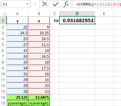
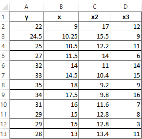
There are the values of x and y:
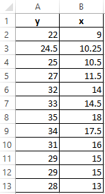
Y is an independent variable, x is an independent variable. It is necessary to find the strength (strong / weak) and the direction (direct / inverse) of the connection between them. The formula of the correlation coefficient looks like that:
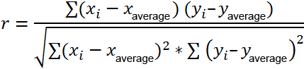
To make it easier to understand, we will break it into several simple elements.
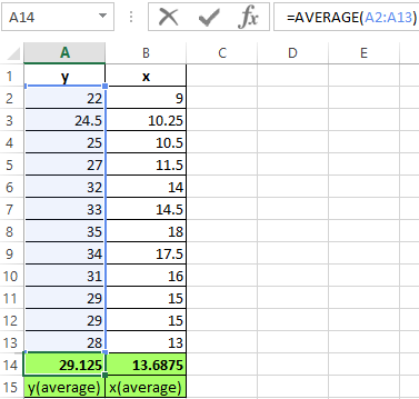
- Find the mean values of the variables using the AVERAGE function:
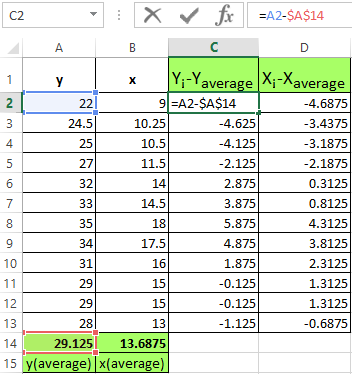
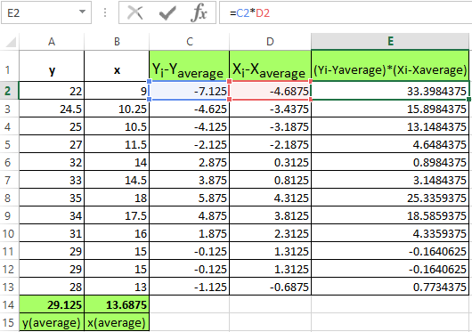
- Calculate the difference between each y and y mean, each x and x medium. We use to the mathematical operator «-».
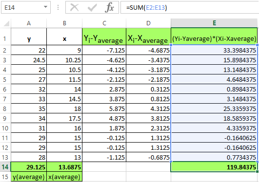
- You need multiply now the differences found:
- Find the sum of the values in this column. This will be the numerator.
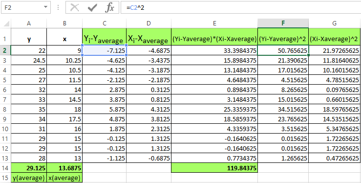
- To calculate the difference denominator of y and y-average, x and x-average. It is necessary to erect it a square.
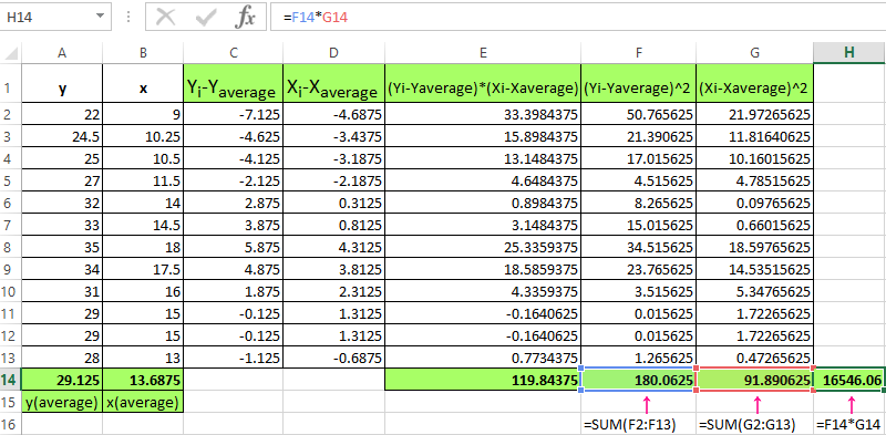
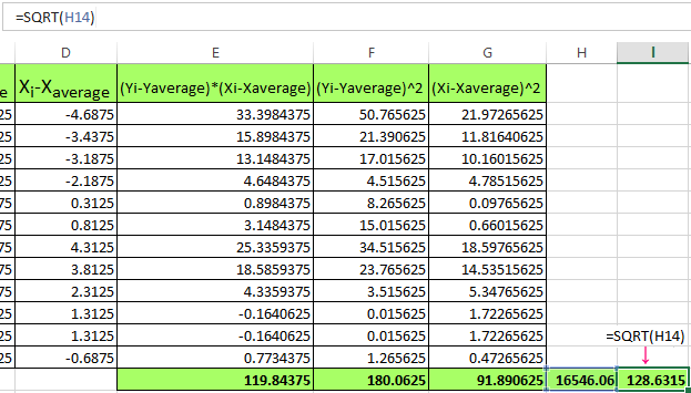
- Find the sum of the values in the received columns (using the AUTO-SUM function) and multiply these values.
- The result is squared (SQRT function).
- It remains to calculate the quotient (the numerator and denominator are already known).
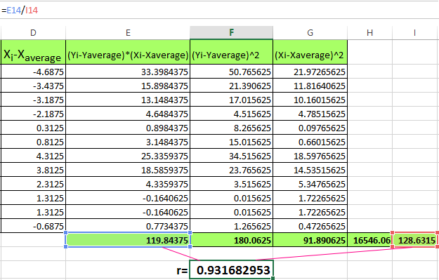
The strong direct link is defined between the variables.
The built-in CORREL function allows you to avoid of complex calculations. We calculate the coefficient of pair correlation in Excel with its help. You need to call the function wizard and to find the right one. The arguments of the function are an array of values of y and an array of values of x:
We show the values of the variables on the chart:
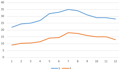
There is a strong interconnection between y and x, because the lines run almost parallel to each other. The interconnection is straight: grows y - grows x, decreases y - decreases x.
The matrix of paired correlation coefficients in Excel
The correlation matrix is the table, at the intersection of rows and columns of which are the correlation coefficients between the corresponding values. It makes sense to build it for several variables.
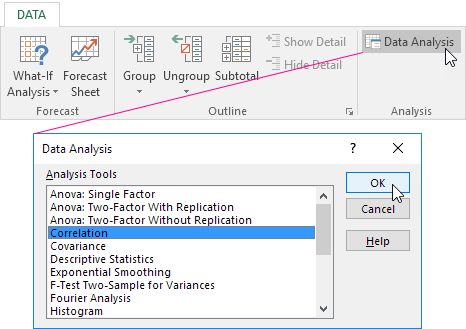
The matrix of correlation coefficients in Excel is constructed using the «Correlation» tool from the «Data analysis» package.
- On the «Data» tab in the «Analysis» group, we need to open the «Data analysis» package (for the 2007 version). If the button is not available, you need to add it («Excel Options»- «Add-ins»). In the analysis tools list, zou need to select «Correlation».
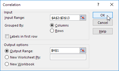
- Click OK and set the parameters for data analysis. The input interval is the range of cells with values. The grouping - by columns (analyzed data are grouped into columns). The output interval is the reference to the cell from which the matrix is to be built. The size of the range will be determined automatically.
- After pressing OK, the correlation matrix appears in the output range. At the intersection of rows and columns there are the correlation coefficients. If the coordinates are the same, the value 1 is output.
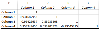
Between the values of y and x1 is found the strong direct connection. There is a strong feedback between x1 and x2. There is practically no connection with the values in the column x3.
Let`s show graphically the correlation relations using graphs.
- The strong direct connection between y and x.
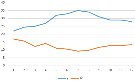
- The strong feedback between y and x2. The values change occur parallel to each other, but if y grows, x falls. The values of y increase - the values of x decrease.
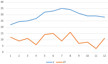
- The absence of the relationship between the values of y and x3. The changes in x3 occur chaotically and its do not correlate with changes in y.
Download calculation coefficient of pair correlation in Excel
Why do we need such the coefficient? It`s need for determining of interconnection between the observed phenomena and forecasting.

Data Visualization Charts for Interactive Report Creation in Excel.
Dashboard Templates