Factor and variance analysis in Excel with automated calculations
The variance method is used to analyze the variance of an attribute under the influence of controlled variables.
The factor method suits for examining the connections between values. Let's consider the analytic tools in detail: namely, the factor, variance and two-factor variance methods for assessing the variability.
Variance Analysis In Excel
In conventional terms, the objective of the variance method is as follows: to single out three particular variances from the general variance of a parameter:
- the variance determined by the influence of each of the values under consideration;
- the variance dictated by the interconnection between the values under consideration;
- the random variance dictated by all the unconsidered circumstances.
Microsoft Excel allows for performing the variance analysis with the help of the tool «Data Analysis» (the tab «DATA» - «Analysis»). It's a customization plugin of the spreadsheet processor. If the plugin is unavailable, go to «Excel Options» and enable the analysis tool.
The work starts with executing the table. The rules are:
- Each column should contain a value of one of the factors under consideration.
- The columns should be organized in ascending/descending order of the value of the parameter under consideration.
Let's review an example of variance analysis in Excel.
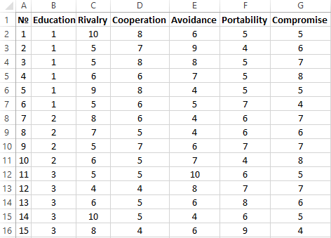
Using a dedicated method, the company's psychologist has analyzed the behavior strategies of employees in a conflict situation. It is assumed that the behavior is influenced by the subject's education level (1 stands for secondary, 2 for vocational, 3 for higher).
Enter the data into the Excel table:
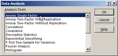
- Open the dialog window of the analytic tool. Select «Anova: Single Factor» in the list and click OK.
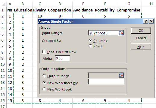
- In the «Input Range» field, enter the link to the range of cells contained in all the table columns $B$2:$G$16.
- Select «Grouped By»-«Columns».
- Select «New Worksheet Ply:» in the «Output options:». If you need to indicate the output range within the existing spreadsheet, switch it to the « Output Range:» and enter the link to the top left cell of the range for the output data. The size of the range will be determined automatically.
- The analysis results are output on a separate spreadsheet (in our example).
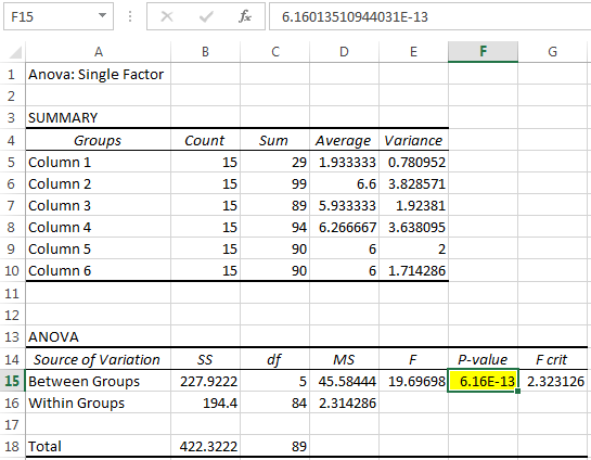
The parameter of importance is filled-in with yellow. As the P value between the groups exceeds 1, Fisher's variance ratio cannot be considered of importance. Consequently, the behavior in a conflict situation does not depend on the subject's education level.
Factor Analysis In Excel: An Example
Factor analysis is a multi-variance analysis of the inter-connections between the values of the variables. This method allows to resolve some very important tasks:
- to describe the object under observation in a comprehensive yet concise manner;
- to reveal the hidden variable values that determine the presence of linear statistical correlations;
- to classify the variables (determining the inter-connections between them);
- to reduce the number of the necessary variables.
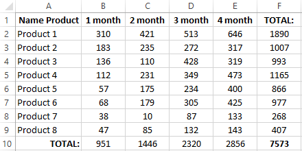
Let's review an example of conducting a factor analysis. Let's assume we know the data regarding the sales of certain goods during the past 4 months. We need to analyze which items are in demand and which are non-demanded.
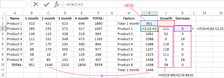
- Let's find out which items ensured the main part of the growth in the second month. If the sales of a certain kind of goods grew, the positive delta goes to the «Growth» column. Negative deltas go to «Decrease». For «Growth», the Excel formula is: =IF((C2-B2)>0,C2-B2,0), where С2-В2 is the difference between the 2nd and 1st months. For «Decrease», the formula is: =IF(J3=0,B2-C2,0), where J3 is the link to the left cell («Growth»). The second column will contain the sum of the previous value and the previous growth, deducting the current decline.
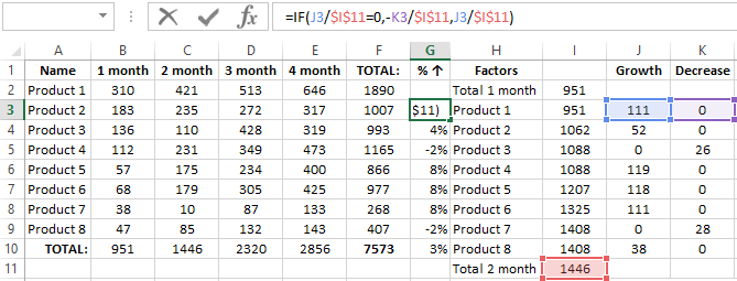
- Let's calculate the growth percentage for each item. The formula is: =IF(J3/$I$11=0,-K3/$I$11,J3/$I$11). Here, J3/$I$11 stands for the ratio between the «Growth» and the result of the 2nd month. ;-K3/$I$11 stands for the ratio between the «Decrease» and the result of the 2nd month.
- Select the range of data for building the chart. Go to the tab «INSERT»-«Chart».
- Let's adjust the legend and the colors. Remove the cumulative total through «Format Data Series» - «FILL» («No fill»). Use this tool to change the colors for «Decrease» and «Growth».
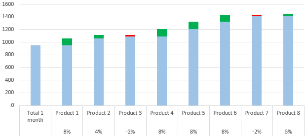
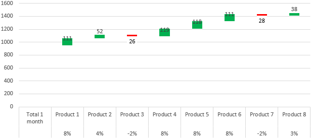
Now we have a visual demonstration of which kinds of goods ensured the main part of the sales growth.
Two-Factor Variance Analysis In Excel
This method demonstrates the influence of two factors on the variance of a random variable's value. Let's consider an example of performing the two-factor variance analysis in Excel.
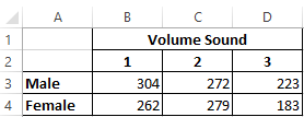
Problem. A group of men and women were demonstrated sounds of various volumes: 1 – 10dB, 2 – 30dB, 3 – 50dB. The response time was recorded in milliseconds. It's necessary to determine: whether or not the subject's sex influences the response time; whether or not the volume influences the response time.
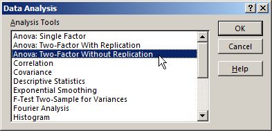
- Go to the tab «DATA»-«Data Analysis». Select «Anova: Two-Factor Without Replication» from the list.
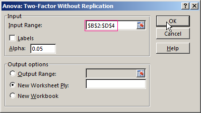
- Fill in the fields. Only numeric values should be included in the range.
- The analysis result should be output on a new spreadsheet (as was set).
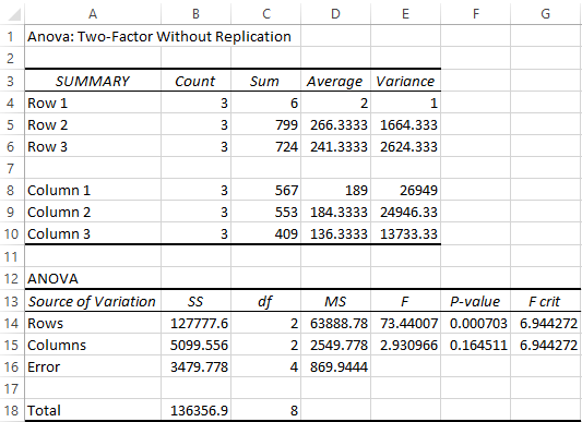
Since the F statistics (the «F» column) for the «gender» factor exceeds the critical level of the F distribution (the column «F-critical »), this factor does have an impact on the parameter under analysis (the time of response to the sound).
As another example, the factor analysis of the deviations in marginal income is provided below:
Download Factor and Variance analysis example
Download analysis example 2For the «Volume Sound» factor: 2,9 < 6,94. Consequently, this factor has no influence on the response time.

Data Visualization Charts for Interactive Report Creation in Excel.
Dashboard Templates