Financial analysis in Excel with an example
Microsoft Excel gives to an user the whole toolkit for analyzing the financial performance of an enterprise, performing statistical calculations and forecasting.
Built-in functions, formulas, add-ins allow you to automate the lion's share of the work. Thanks to automation, an user needs only to substitute new data and on their basis automatically generated ready reports, which a lot of people make for hours.
The example of the financial assay of the company in Excel
The task – is to study the results of financial activities and the state of the company. There are objectives:
- to evaluate the market value of the firm;
- to identify ways of effective development;
- to analyze solvency, creditworthiness.
Based on the results of financial activities, the manager develops a strategy for further development of the company.
The analysis of the financial condition of the company implies:
- the assay of the balance and the income statement about profits and losses;
- the analysis of liquidity of the balance sheet;
- the analysis of solvency, financial stability of the enterprise;
- the analysis of business activity, the state of assets.
Let`s consider the methods of analyzing the balance sheet in Excel.
First we make the balance (for example – schematically, not using all the data from the Form 1).
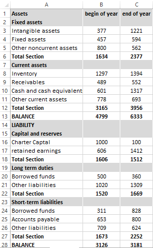
Let's analyze the structure of assets and liabilities, the dynamics of changes in the value of the articles - we will construct the comparative analytical balance.
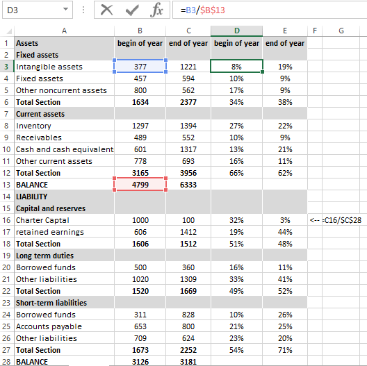
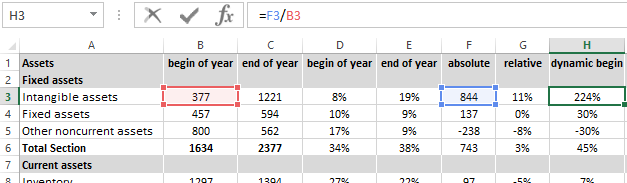
- Let's imagine the values at beginning and end of an year in the form of relative values. There is formula: = B4 /$B$14 (the ratio of the value at beginning of the year to the value of the balance at the beginning of the year). By the same principle, we formulate formulas for «end of the year» and «passive». Copy in the entire column. In the new columns, you need to set the percentage format.
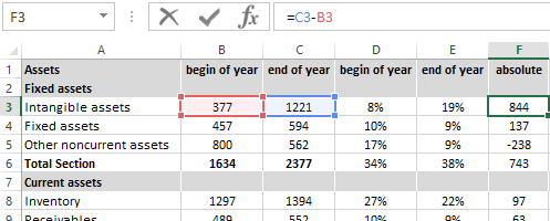
- Let`s analyze the dynamics of the changes in absolute values. We make the additional settlement column, in which we will reflect the difference between the value at end of the year and beginning.
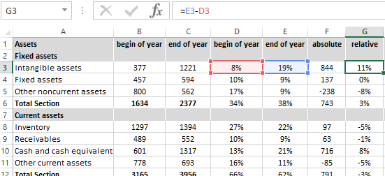
- Let's show the changes in the relative values. In the new calculated column, we find the difference between the relative indicators of the end of the year and the beginning.
- To find the dynamics in percentage to the value of the indicator of beginning of the year, we consider the ratio of the absolute indicator to the value of beginning of the year. There is the formula: = F4/B4. You need to copy in the entire column.
- By the same principle, we find the dynamics in percent for the end-of-year values.
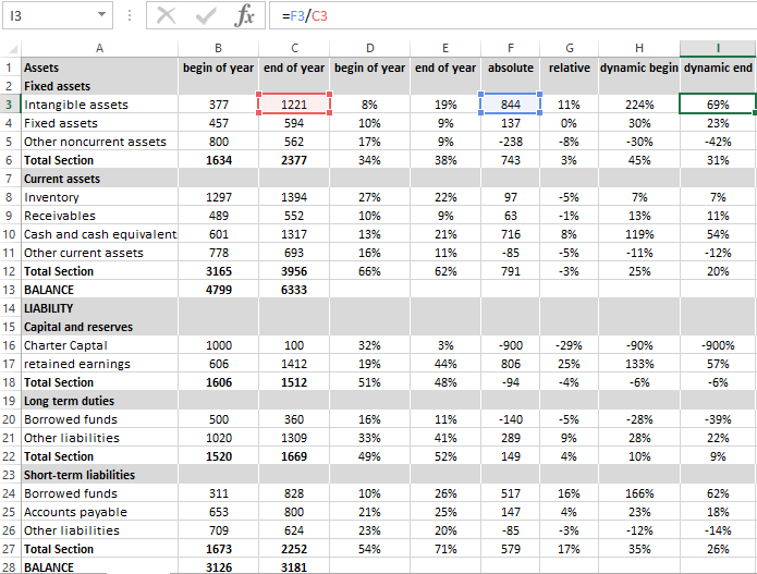
With the helping of the simplest formulas, we have shown the dynamics of the balance sheet items. In the same way, you can compare the balances of different enterprises.
What are the results of the analytical balance?
- The balance currency at the end of the accounting period has become larger in comparison with the initial period.
- The non-current assets are incremented at a higher rate than negotiable assets.
- Own capital of the enterprise is more than borrowed one, in which connection growth rate of its own exceed the dynamics of borrowed capital.
- The accounts payable and receivable are growing at approximately the same pace.
The statistical analysis of data in Excel
To implement of the statistical methods in Excel there is the huge set of tools is provided. Some of them – are built-in functions. Specialized methods of data processing are available in the «Analysis package» Add-on.
Let`s consider the popular statistical functions.
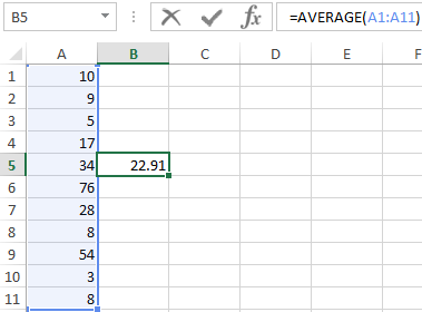
- AVERAGE – Average value – calculates the sample or general average. The argument of the function is the set of numbers specified as the reference to a range of cells.
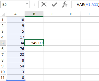
- VAR– for calculating of the sample variance (without taking into account text and logical values); VARA - takes into account text and logical values. VARP (VAR.P) – for calculating the general variance (VARPA - with taking into account text and logical parameters).
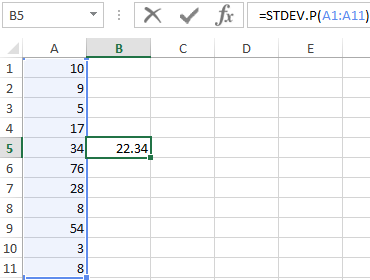
- For finding the square root of the variance – STDEVP (STDEV.P)(for selective standard deviation) and STDEVPA (for the general standard deviation).
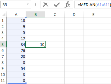
- For finding the mode of the data set, the function of the same name is used. It divides the data range into two equal parts of the MEDIAN by the number of elements.
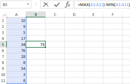
- The range of variation – is the difference between the largest and the smallest value of the data set. You can find Excel in the following way:
- To check the deviation from the normal distribution allow the functions of the SKEW (asymmetry) and KURT. The asymmetry reflects the amount of asymmetry in the distribution of data: the most of the values are greater or less than the mean.
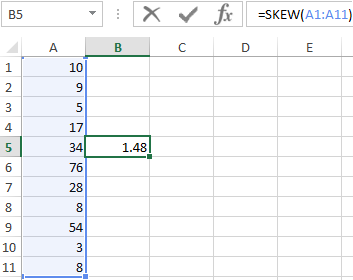
In the example most of the data is above average, because the asymmetry is greater than «0».
KURT compares the maximum of the experimental with the maximum of the normal allotment.
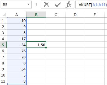
In the example the maximum distribution of the experimental data is higher than the normal distribution.
Let's consider how the «Analysis package» add-on is used for statistical purposes.
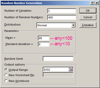
The task: to generate 400 random numbers with normal distribution. To complete the list of statistical characteristics and histogram.
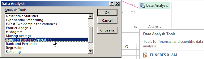
- Let`s open the menu of the «Data analysis» instrument in the «Data» tab (if this tool is not available, you need to connect the analysis Add-Ins). Let`s choose the line «Random Number Generation».
- We enter the following data in the dialog box fields:
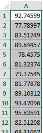
- After clicking OK:
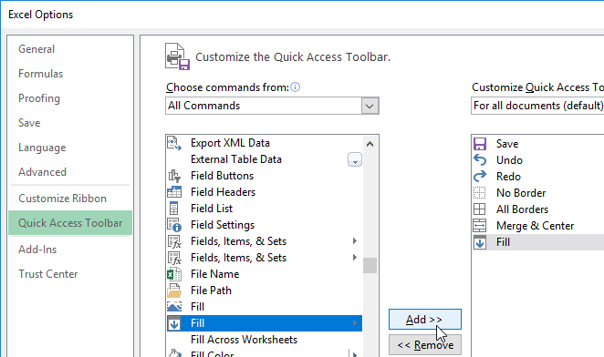
- We define the solution intervals. Let`s suppose that their lengths are the same and equal by 3. We put the cursor in the cell B2. Enter the initial number to automatically compile of the intervals. For example, is 65. Next, you need to make the «Fill» command available. Open the «Excel Options» menu (the «FILE» button). We perform the actions are shown in the picture:
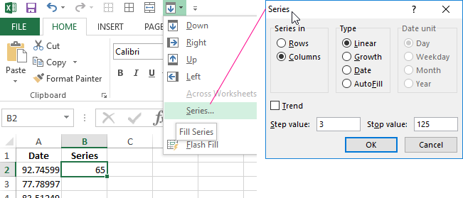
- The desired button appears in the Quick Access toolbar. In the drop-down menu, you need to select the «Series» command. We fill the dialog box. The B column will show break intervals.
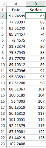
- The first result of the work:
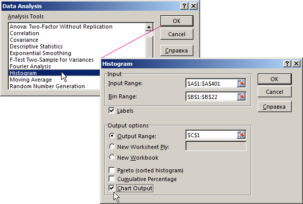
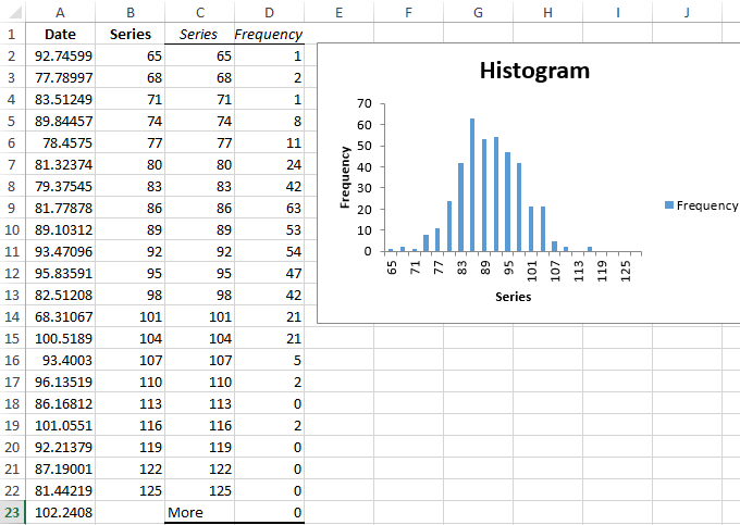
- We open the list of the tool «Data analysis» again and choose the «Histogram». Fill in the dialog box:
- The second result of the work:
- The «Descriptive Statistics» command (Data Analysis package) will help you to build a table of statistical characteristics. The dialog box is filled in the following way:
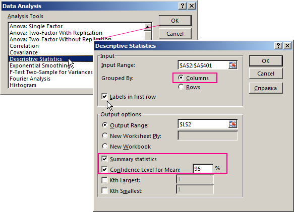
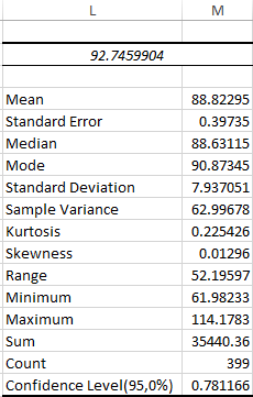
After pressing OK, the basic statistical parameters for this row are displayed.
Download an example of financial analysis in Excel
This is the third final result of the work in this example.

Data Visualization Charts for Interactive Report Creation in Excel.
Dashboard Templates