Timekeeping Spreadsheet Tracking in Excel - Free Download
Timekeeping sheet is a key document containing information about the attendance and absence of each employee in the company. It is submitted to the accounting department, and based on the data, salaries are calculated and awarded.
There are two standardized forms of timekeeping defined by law: T-12 for manual entry and T-13 for automatic monitoring of actual working hours (via turnstile).
Data is entered every working day. At the end of the month, the total for attendance and absence of each employee is calculated. Automating the filling of certain cells in Excel can simplify report generation. Let's see how.
Filling in Initial Data with Excel Functions
Forms T-12 and T-13 have practically the same set of requisites.
In the header of the second page of the form (using T-13 as an example), fill in the name of the organization and structural unit, as specified in the founding documents.
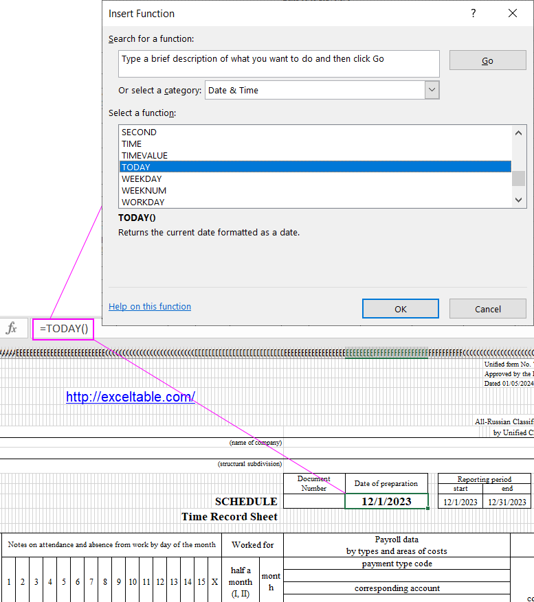
Manually write the document number. In the "Date of Preparation" column, set the TODAY function by selecting the cell, finding the function in the list, and clicking OK twice.
In the "Reporting Period" column, specify the first and last dates of the reporting month.
Allocate a space beyond the time sheet on a separate sheet named "Directory." This is where we will work. First, create a calendar for the reporting month.
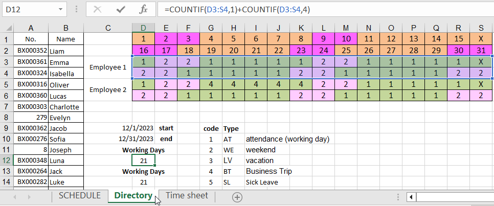
Orange field - dates. In the green field, mark ones for weekends. In cell T2, put one if the time sheet is for the entire month.
For highlighting weekends with magenta color, use a conditional formatting formula that refers to the dates specified in the document:
=OR(WEEKDAY(DATE(YEAR($D$9),MONTH($D$9),D1))=1,WEEKDAY(DATE(YEAR($D$9),MONTH($D$9),D1))=7)
Determine the number of working days in the month for each employee and consider business trip days with code 4. Do this in the operating field. Insert the formula into the necessary cell:
=COUNTIF(D3:S4,1)+COUNTIF(D3:S4,4)
The COUNTIF function counts the number of non-empty cells in the specified range.
Manually enter the serial number, full name, and job title of the organization's employees, plus their employee ID. Retrieve this information from the employees' personal cards.
Automating the Time Sheet with Formulas
The first sheet of the form contains symbols for tracking working hours, both numeric and alphabetic. The goal of automating with Excel is to display the number of hours when a symbol is entered.
For example, we'll take these variants:
- AT - attendance (working day)
- WE - weekend
- LV - vacation
- BT - Business Trip
- SL - Sick Leave
First, use the CHOOSE function. It allows you to set the desired value in a cell. At this stage, we'll need the calendar we created in the Operator Field. If a day is a weekend, "WE" appears in the time sheet. "AT" indicates a working day. Example:
=CHOOSE(Directory!$D$3,"AT","WE","LV","BT","SL")
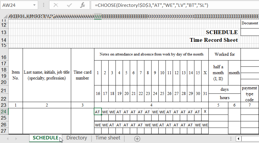
Enter the formula into one cell, then drag it from the lower right corner and apply it to the entire row.
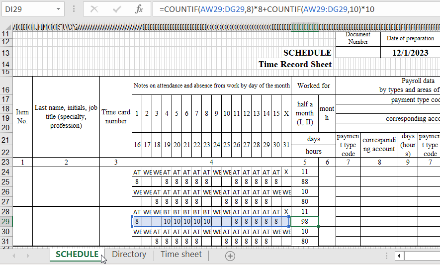
Now, let's ensure that employees' working days are marked with "eights." Use the IF function. Select the first cell in the row under symbols. Insert the function: IF logical test - the address of the cell being converted (the cell above) = "AT". If true - 8; otherwise, a nested IF function to check the second condition: if = "BT" - 10; else, "" (empty). If it's indeed a weekend, 0 working hours. Drag the lower right corner of the cell with the formula and replicate it across the entire row.
Repeat the same process for the second half of the month and subsequent employees. Simply copy the formulas and change the cells they reference.
Now, let's summarize: calculate the number of attendances for each employee. Use the COUNTIF formula. The range for analysis is the entire row where we want to get the result. The criterion is the presence of the letter "AT" (attendance) or "BT" (business trip) in the cells. Example:
=COUNTIF(AW24:DG24,"AT")+COUNTIF(AW24:DG24,"BT")
This result gives the number of working days for a specific employee.
Calculate the number of working hours. There are two ways: a simple one using the SUM function, and a more complex but reliable one using the COUNTIF function. Example formula:
=COUNTIF(AW25:DG25,8)*8+COUNTIF(AW25:DG25,10)*10
Where AW25:DA25 is the range, the first and last cells of the row with the number of hours. The criterion for a working day ("AT") is "=8". For a business trip ("BT") - "=10" (in our example, 10 hours are paid). The result after entering the formula:
 Download timekeeping sheet in Excel
Copy all the formulas and paste them into the corresponding cells throughout the employee list. When filling out such a time sheet, you will need to adjust the symbols for each employee.
If the calendar changes, weekends and attendances change as well. Manually mark absences, compensatory days off, etc. Everything else will be calculated automatically.

Data Visualization Charts for Interactive Report Creation in Excel.
Dashboard Templates