How to find Identifying Duplicate values in Excel column?
The searching of duplicates in Excel – is one of the most common tasks for any of office employee. For its solution, there are a few different methods. But – how quickly to find duplicates in Excel and to highlight them with color? For the answer on this frequently asked question let us consider a concrete example.
How to find duplicate values in Excel?
For example we are engaging by check orders, which coming into the firm through Fax and e-mail. There can be such situation that the same order was by the two channels of incoming information. If you register twice the same order, there can be certain problems for the firm. Below we are considering to the decision by means of the conditional formatting.
For avoiding of the duplicate orders, you can use to the conditional formatting, which helps you quickly to find the duplicate values in Excel column.
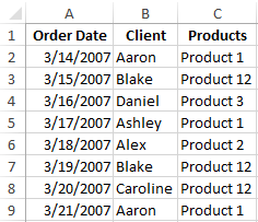
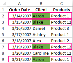
The example of the day orders for goods:
For verification whether the day orders are possible duplicates, we will analyze in the names of customers – there is the column B:
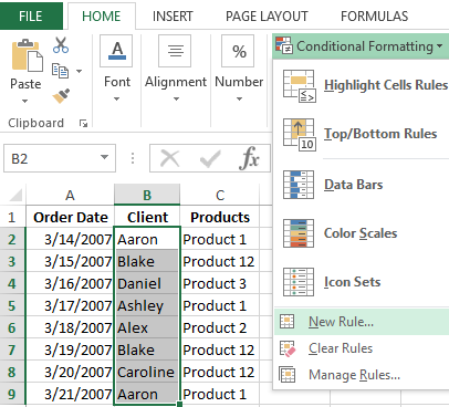
- To highlight the range B2:B9 and then to select the instrument: «HOME» - «Styles» - «Conditional Formatting» - «New Rule».
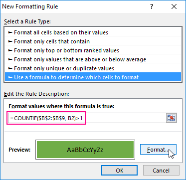
- To choose «Use a formula to determine which cells to format».
- To find the duplicate values in Excel column, you need to enter the formula in the input field:
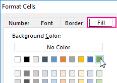
- After that you need to press the button «Format» and select to the desired cell shading to highlight duplicates in color - for example, green one. And click OK on all windows are opened.
Download an example of finding the Identifying Duplicate values in a column.
As can be seen in the picture with the conditional formatting we were able easily and quickly to implement the duplicate finder in function Excel and to detect to the duplicate data cells for the table of the day orders.
The example of COUNTIF function and highlighting of the duplicate values
The principle of the action formula for finding of the duplicates by the conditional formatting is simple. The formula contains the function =COUNTIF(). This function can also be used when searching for the identical values in the range of cells. The first argument in the function to the viewable data range is specified. In the second argument we specify what we are looking for. The first argument has an absolute reference, as it should be the same one. And the second argument conversely - should be changed on the address of the each cell in the viewing range, because it has a relative link one.
The fastest and the simplest ways: to find to the duplicates in the cells.
After the function we can see the comparison operator of the number of the found values in the range with the number 1. That is, if we see more, than one value means that the formula returns the value of TRUE and for the current cell is applied to the conditional formatting.

Data Visualization Charts for Interactive Report Creation in Excel.
Dashboard Templates