Searching of the value in a range Excel table in columns and rows

Let suppose that your report contains a table with lots of data in many columns. To conduct the visual analysis of such tables is extremely difficult. And one of the tasks to work with the report - there is the analysis of the data relative to the rows and column headers for a particular month. At first glance this is a very simple task, but it cannot be solved using a standard function.

Yes, of course you can use the tool: «HOME» - «Edit» - «Find» CTRL+F to invoke to the search window values in the Excel worksheet, or create for the table the conditional formatting rule. But then, you cannot perform further calculations with the results obtained. It is therefore necessary to create and correctly apply to the appropriate formula.

The searching of the value in Excel array

The scheme of the solution of the task looks like this:

in the cell B1 we will enter the required data;
in the cell B2 will be displayed the title of the column that contains the value of cell B1;
in cell B3 will be displayed to the name of the row that contains to the value of the cell B1.

In fact you need to search coordinates in Excel.

For what is it need? Quite often we need to get the coordinates of the table – it`s a bit like a reverse matrix analysis. The specific example in a nutshell looks like this: the goal in numbers is the starting value, you need to determine who and when is the closest to this goal. For example, let's use the simple data matrix with the report on the number of goods are sold for three quarters, as shown in the picture below. It is important that all the numbers are match. If you do not want to manually create and populate to the Excel table with a clean sheet, at the end of the article you can download it with an example.

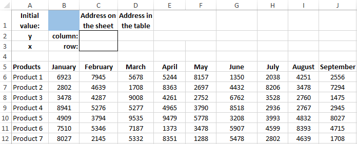
Let`s consider the sequence of the solutions of varying complexity, and at the end of the article we will receive to the final result.

The search of the value in Excel column

Primarily we learn how to have to the table column headers. For this do the following:

In the cell B1, enter the value which was taken from the table 5277 and highlight its background in blue for readability of the input field (we will enter in the cell B1 other numbers, that to experiment with new values).
In the cell C2 we enter to the formula for retrieving the column header of the table which contains this value:

After entering of the formula for confirmation you need to press the hot key combination CTRL + SHIFT + Enter, because the formula must be executed in the array. If you do everything correctly, in the edges of the formula bar will appear braces { }.

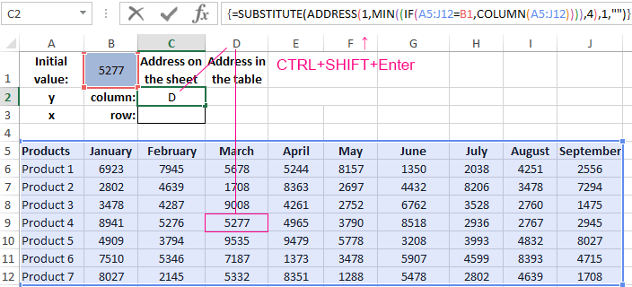
In the cell C2, the formula returned the letter D - the corresponding column header of the sheet. As you can see everything to come together, the value of 5277 contains in the cell of the column D. We recommend looking at the formula to get the whole address of the current cell.

Search values in the row Excel

Now we get to the row number for that value (5277). To do this, in the cell C3 you need to enter the following formula:

After entering of the formula for confirming, you need to press CTRL + SHIFT + Enter again and getting to the result:

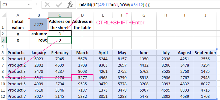
The formula returned to the number 9 and found to the row header of the sheet by the corresponding value in the table. As a result, we have to the full address value D9.

How to get the column title and the title of row in the table

Now we are learning how to get the value the coordinates are not whole sheet, and the current table is. In short, we need to find the value of 5277 instead of D9 to headers:

for the table column – is March;
for the row – the Item 4.

For solving of this task we will use to the formula with already obtained the values in the cells C2 and C3. For this we are doing so:

For the column header: in the cell D2 you need to enter the formula:

At this time after entering of the formula for confirming you need to press as a tradition just Enter:

For the row we input the similar one, but a slightly different formula:

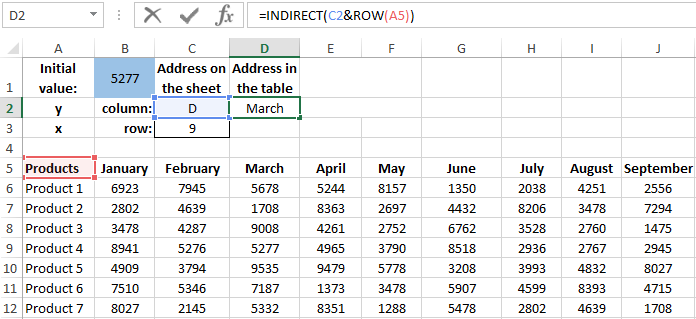
In the result we receive to the internal coordinates of the table by value – March; the Item 4:

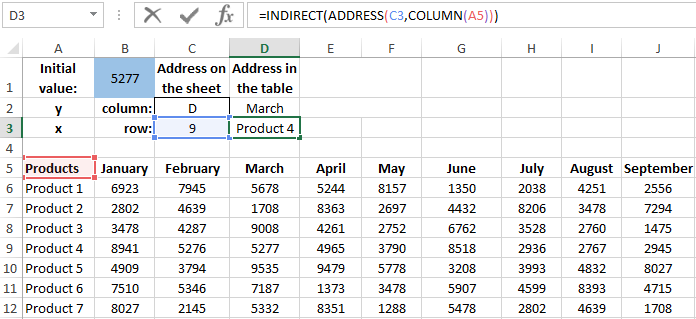
At first glance everything works fine, but what if the table contains 2 of the same values? Then you can have problems with mistakes! We also recommend looking at an alternative solution for searching for columns and rows by value.

The searching for duplicate values in the range Excel

For checking to the duplicates among of the values of the table, we are creating to the formula that will be able to inform us about the presence of duplicates and count their number. To do this, in the cell E2 we enter to the formula:

Moreover, for the range of the table part we are creating the rule of conditional formatting:

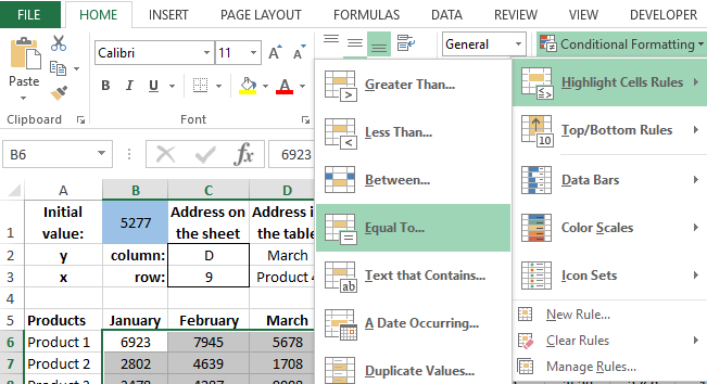
To select the range B6 : J12 and click to the tool: «HOME»-«Styles»-«Conditional formatting»-«Highlight Cells Rules»-«Equal To».

In the left box you need to enter the value $B$1, and from the right drop-down list to select «Light red fill and dark red color» and press OK.

In the cell B1 you need to enter the value of 3478 and admire to the result.

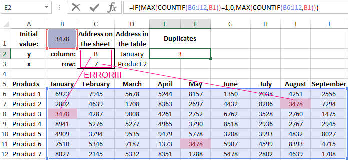
As we can see if you have of the duplicates, the formula for the headings takes the title from the first of the duplicate horizontally (from left to right). And the formula for receiving of the name (number) of the row takes the number from the first of the duplicate vertically (top to bottom). To remedy this solution there are 2 ways:

To obtain the coordinates of the first duplicate horizontally (from left to right). For this in the cell C3 only you should change the formula to: In the result we receive to the correct coordinates for both the sheet and the table:

To obtain to the coordinates of the first duplicate vertically (top to bottom). To do this, you should change in the cell C2 to the formula to:

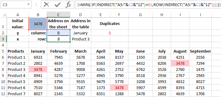
In this case, change the formula either one or the other, but not in two at once. It is worth recalling that in the cell C3 needs to be the old formula:

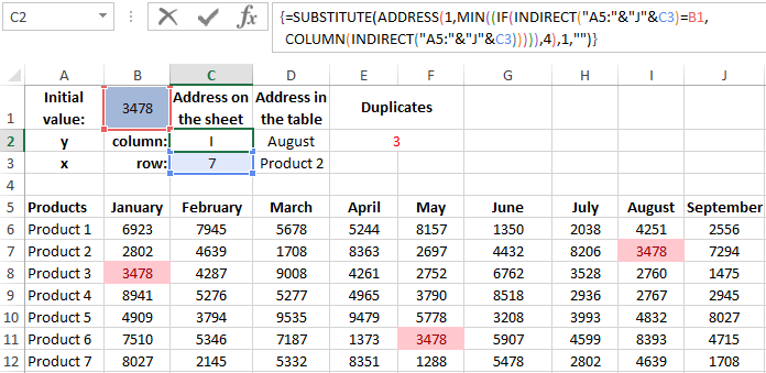
Here correctly displays the coordinates of the first duplicate vertically (from the top to the bottom) – I7 for the list and August; the Item 2 for the table. Let's leave this option for the following final example.

The searching of the nearest value in Excel range

This table is not still perfect, because in the analysis you need to know exactly all the values. If the number entered in the cell B1, the formula does not find in table then the error is returned – #VALUE! It would be ideally, that the formula in the absence of the table of the original number will picked up itself to the nearest value which the table contains. To create such program for the analysis in the table into the cell F1, you need to enter the new formula:

After which you should in all other formulas to change the reference to B1 is supposed to be F1! You also need to change the reference in the conditional formatting. To select: «HOME» -«Styles» - «Conditional formatting» - «Manage rules» -«Change rule», and here in the parameters to enter F1 instead of B1. For testing the program, enter in the cell B1 to the number of which is not in the table, for example: 8000. This will lead to the final result:

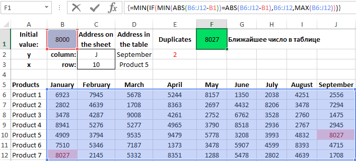
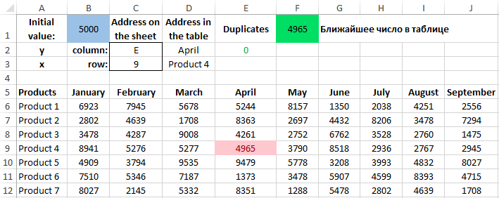
Now you can enter any initial value, and the program will select itself the nearest number that contains the table then displays the column title and the row title for the current values. For example, if you enter 5000 you will get a new result:

Download the example of finding values in the range Excel

Our program in Excel will find the closest value 4965 to the original 5000. This program can be useful for the automatically solving of the different analytical tasks in business-planning, goal setting, finding a rational solution, etc. And the resulting rows and columns allow you to further expand to the computational capabilities of such reports using with helping the new Excel features.