Data Smoothing Formula Using Moving Average Method in Excel
Data smoothing involves eliminating or reducing individual values containing statistical anomalies. The moving average can be used to reduce the influence of unusually high or low values on the result. With a moving average, an informative trend line for all statistical values emerges. The moving average is especially useful for filtering out isolated erroneous values.
How to Find the Moving Average in Excel
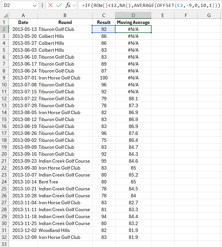
Below is an image showing part of the result list of a golf match. Anyone who plays this game knows that erroneous results can carry over from one round to the next.
The next image shows a graph of the results over time:
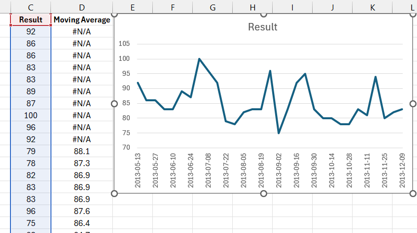
It's difficult to determine the trend of the game based on the values of this graph due to the sharp rises and falls in the curve.
How to Build a Moving Average on a Graph in Excel
Suppose we need to build a graph that, by smoothing sharp rises and falls in the curve, clearly shows the trend in the match results. To smooth the graph, we need to calculate the moving average (MA) for the results and plot it on the graph.
Below is an image of a graph with a moving average curve. It is based on the values in the third column of the table, where the formulas for its calculation are located. The original match results are shown as a thin blue line:
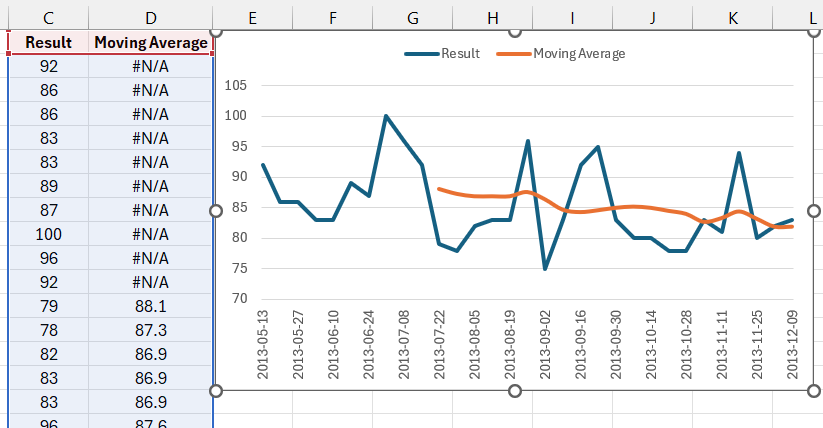
As you can see in the image, thanks to the moving average, we can not only identify the current downward trend but also observe its relatively low dynamics within 5 points along the Y-axis.
The following formula was used to create a new dataset containing MA values for all the original results:
=IF(ROW()<12,NA(),AVERAGE(OFFSET(C2,-9,0,10,1)))
This formula uses several Excel functions. First, the IF function is used, which returns the #N/A! error for the first few results. The ROW function without arguments returns the row number of the sheet for the current cell. It is impossible to calculate the moving average if there are not enough data, so for the first nine values, the formula returns the #N/A! error.
We also recommend that you familiarize yourself with how to calculate using the Excel formula Exponential Moving Average.
Note. The #N/A! error is not displayed on the graph. When Excel encounters errors at the beginning of the data, it does not plot anything, and you can use the NA function, which returns the #N/A! error. However, in the middle of the curve, Excel ignores the errors, creating a continuous line. To make it break in the right places, you need to manually delete the values or use a macro in the corresponding spots. It is impossible to solve this with a formula since any formula will return some result, even an empty string (""). On the graph, it will be displayed as a line, as with a value of 0.
The AVERAGE function is used to calculate the average of the previous 10 game results. This function can take a maximum of 255 arguments, but in this example, the original values form a range, so it is enough to fill in just one argument by specifying the reference to the original cell range.
The OFFSET function returns a selected cell range shifted by 10 cells from the original range each time. This function contains the following arguments:
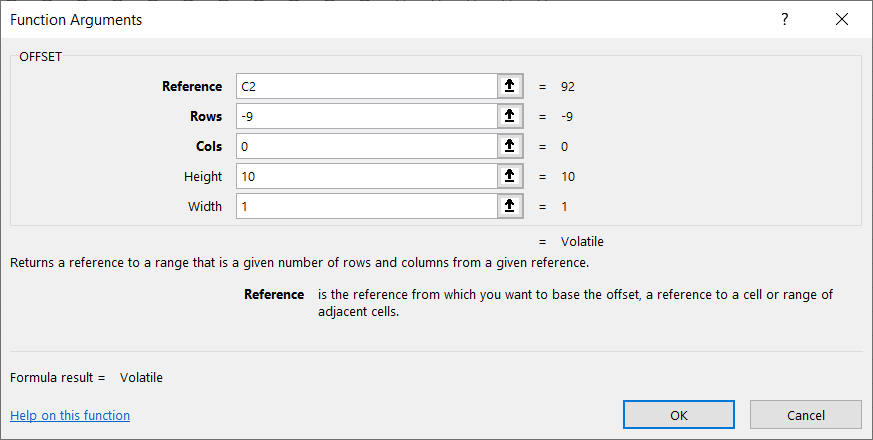
- Reference – the address of the cell from which the function begins its calculation for the offset.
- Rows – specifies the number of rows between the starting cell and the beginning of the returned range. A negative number means the returned range is above the starting cell, and a positive number means it is below.
- Columns – specifies the number of columns between the starting cell and the beginning of the returned range. A negative number means the range is to the left, and a positive number means it is to the right.
- Height – the number of rows in the returned range (must be a positive number).
- Width – the number of columns in the returned range (must be a positive number).
Download an Example of How to Find the Moving Average in Excel 
If the reference argument for the OFFSET function is set to C11, it will begin counting rows and columns from that point in the Excel sheet. The negative number -9 as the second argument (Rows) will move the reference up 9 rows to cell C2. The third argument (Columns) is set to 0, meaning the function will not move horizontally. Based on these two arguments, the function will calculate that the returned range begins at C2.
The 4th argument (Height) is set to 10, meaning the returned range has a height of 10 rows, covering cells C2:C11. The 5th argument (Width) is set to 1, meaning the returned range consists of 1 column. As a result of these calculations, the OFFSET function returns a reference to the new cell range C2:C11, which is passed as an argument to the AVERAGE function. As the formula is copied to subsequent cells, the previous 10 game results are averaged.
In this way, MA line for the match results graph was calculated. MA, based on the arithmetic mean of the previous 10 match results, made the graph more readable. Now the trend direction for the golf match results is clearly visible.
The number of values considered in MA can vary depending on the original data and the task at hand. You can average values over the last 12 months, 5 years, or any other period relevant to the data.
