Example of a Formula for Sales Deseasonalization in Excel
Sales data over one or more years always contain periods of seasonality. This means that sales during certain times of the year are higher or lower than average. An important element of data programming is accounting for their seasonality.
How to Calculate Sales Deseasonalization in Excel Using a Formula
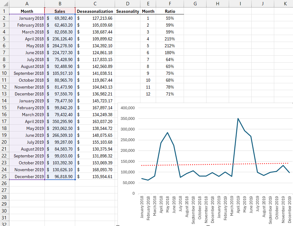
The chart below shows sales data over a five-year period. The chart also includes a trendline showing a constant increase in sales. The most important feature of the chart is the sharp rise in sales during late spring and early summer. If you try to forecast data based solely on the trendline, the store would likely lack staff and stock during the hot sales season:

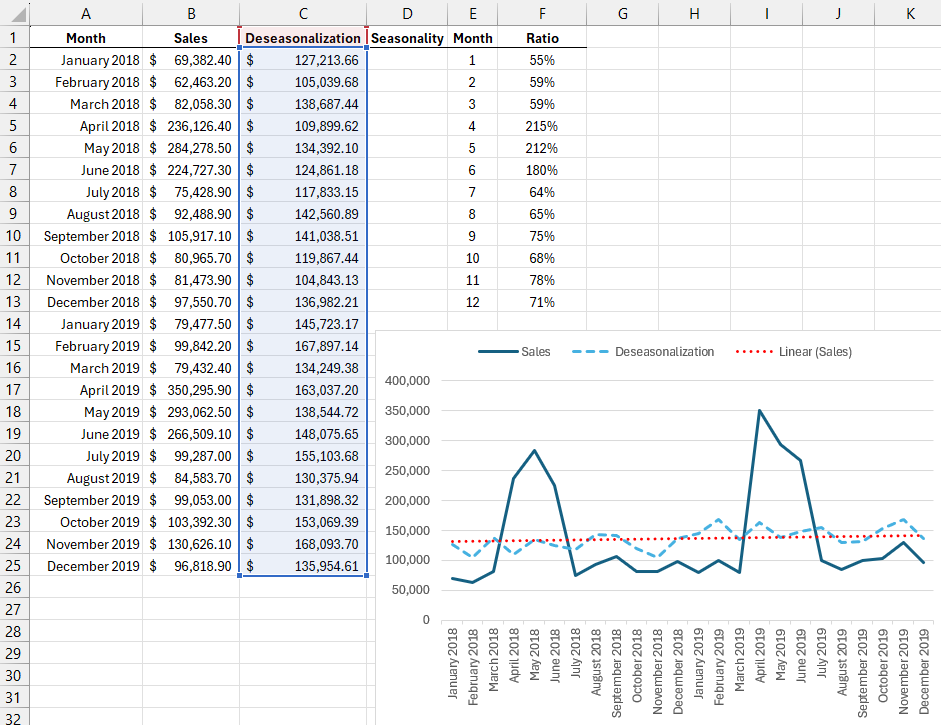
To properly forecast and plan sales for the upcoming year, you should deseasonalize the data. After that, determine the trend for the deseasonalized data and then re-establish the seasonality.
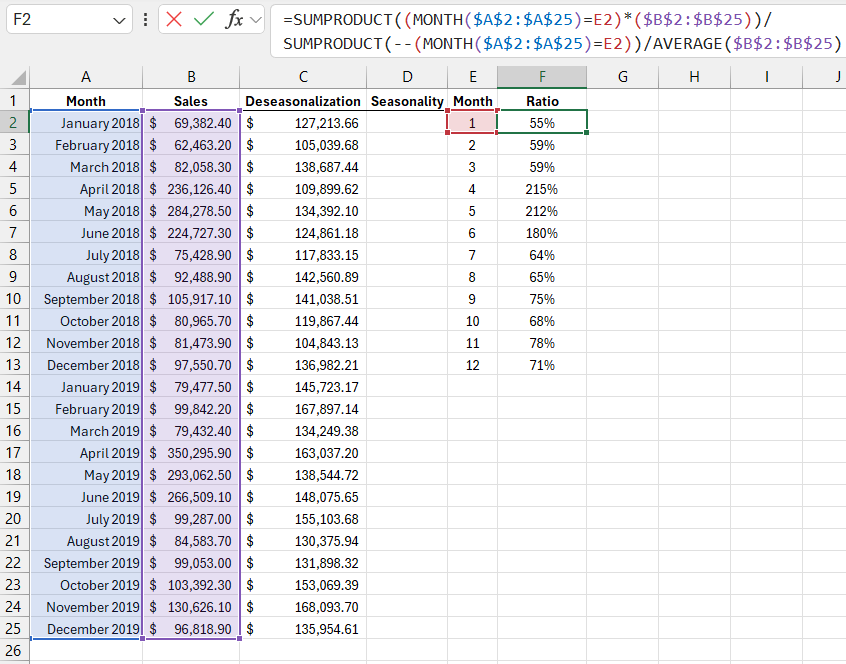
The table below (E1:F13) contains month numbers and their corresponding seasonality coefficients. This coefficient shows how much sales in a given month deviate from the overall average. The table illustrates that January sales are about half of the average value (55%), while April sales are more than double (215%). To calculate the seasonality coefficient, the following formula is used:
=SUMPRODUCT((MONTH($A$2:$A$25)=E2)*($B$2:$B$25))/SUMPRODUCT(--(MONTH($A$2:$A$25)=E2))/AVERAGE($B$2:$B$25)

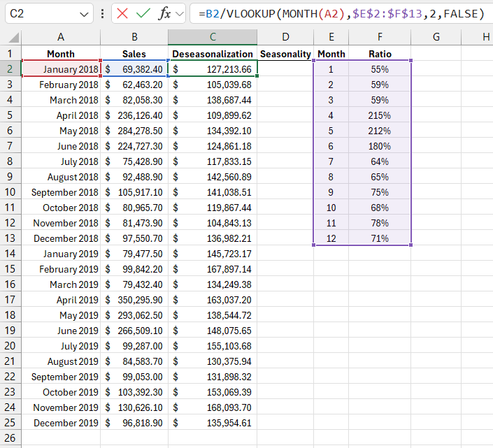
To perform the deseasonalization, the column next to the sales data was filled in with values. In this column, each month's sales were divided by the seasonality coefficient, yielding the deseasonalized value. The formula for deseasonalizing sales data looks like this:
=B2/VLOOKUP(MONTH(A2),$E$2:$F$13,2,FALSE)

The chart shows that, had there been no seasonality, January 2018 sales would have been 127,213.66.

Formula for Calculating the Sales Seasonality Coefficient in Excel
The formula that calculates the seasonality coefficient uses two SUMPRODUCT functions, which compute the average sales for the month specified in the adjacent cell. The average sales for that month are divided by the overall average sales.
The first SUMPRODUCT function sums all values in the range B2:B25 where the cells in the range A2:A25 contain the month number equal to the one in cell E2. The formula in cell F2 sums the sales figures for January each year.
The second SUMPRODUCT function counts the occurrences of January in the range A2:A25. SUMPRODUCT returns an array of TRUE or FALSE values. The double negative sign converts these values into 1 (for TRUE) and 0 (for FALSE). SUMPRODUCT then sums all the 1s and returns the count of January occurrences in the dataset.
Dividing the result of the first SUMPRODUCT calculation by the result of the second function gives the sum for each January divided by the number of occurrences. This average value is then divided by the overall sales average to return the seasonality coefficient.
Download Example of Sales Deseasonalization in Excel 
Finally, the sales figures for each month are divided by the seasonality coefficient. To find the coefficient in the table, the VLOOKUP function is applied. The lookup value is determined using the MONTH function, which returns the month number.
Continue Reading: FORECAST Formula for Sales Prediction Considering Seasonality in Excel
This value is then compared with the values in the first column of the table.
