Excel Formula for Weighted Average Interest Rate of Portfolio
The weighted average is used to calculate the average of statistical values that have different (higher or lower) values within a dataset.
Example Formula for Calculating the Weighted Average Interest Rate in Excel
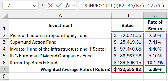
Suppose we need to determine the weighted average interest rate of an investment portfolio. Below is an image of the complete investment portfolio. For each investment, the value and return rate are indicated. Let's assume we need to calculate the overall portfolio return rate. To determine the portfolio’s return rate as a percentage, we use the following formula:
Source Data Table:
| Investment | Value | Rate of Return | Investment Share | Return Share |
| Pioneer Eastern European Equity Fund | $72,021.35 | 2.50% | 17% | 0.43% |
| Superfund Action Fund | $25,419.31 | 7.41% | 6% | 0.44% |
| Investor Fund of the Infrastructure and IT Sector | $97,440.65 | 4.40% | 23% | 1.01% |
| ING European Dividend Companies Fund | $88,967.56 | 5.10% | 21% | 1.07% |
| Kazna Top Brands Fund | $139,806.15 | 10.12% | 33% | 3.34% |
| Weighted Average Rate of Return: | $423,655.02 | 6.29% | 6.29% |
=SUMPRODUCT((B2:B6/B7),C2:C6)

To calculate the weighted average interest rate, the proportion of each investment in the total portfolio value is multiplied by its return rate. The SUMPRODUCT function is ideal for multiplying two sets of data (arrays) and then summing the results. This function can take up to 255 arguments, separated by semicolons. However, in this formula, we only need to use two arguments.
The first argument contains the values of all investments, divided by their total, giving five percentage values that represent the weight of each investment in the portfolio. For example, the fund “Pioneer Eastern European Equities” accounts for 17%, calculated by dividing 72,021.35 by 423,655.02. The second argument contains the return rates for each investment. The SUMPRODUCT function multiplies each element from the first argument by the corresponding element in the second argument. The element B2/B7 is multiplied by C2, B3/B7 by C3, and so on. After multiplying all five elements, the function sums the results.
If we had used the AVERAGE function to calculate the average return rate, the result would have been 5.906%. However, this is lower than the weighted average interest rate of the portfolio. For instance, the "Kazna Top Brands Fund" has both a high return rate and a larger share of the portfolio than other positions.
How to Calculate the Weighted Average Interest Rate in Excel Step by Step
In the above example, all calculations are performed using the SUMPRODUCT function to calculate the weighted average. These calculations can also be done using basic functions entered into adjacent cells. Below is an image showing the same calculations as in the previous example, but instead of using the SUMPRODUCT function, a different method is used. The share of the portfolio for each individual investment is calculated in separate cells, followed by the contribution of each return rate to the final result. Finally, the results are summed using the basic SUM function.

Download Example of How to Calculate Weighted Average Interest Rate of Investment Portfolio in Excel 
Excel is the most versatile analytical tool, well-suited for performing statistical data analysis. It includes a vast array of specialized statistical functions. Next, we will explore formulas used for analyzing statistical data, such as averaging, segmentation, or building frequency charts.
