How to Approximate Search with Inexact Match in Excel
For Excel lookup functions such as VLOOKUP, HLOOKUP, and MATCH to perform an exact search and return either the exact match of the search value and the checked cell value, or an error, the third argument must be set to FALSE or 0. This applies regardless of whether the list of values being searched is sorted or not.
Formula for Approximate Search with Inexact Match in Excel
Excel’s lookup functions designed to retrieve values from tables can also find data when an approximate value is needed. However, this only works with lists of values sorted in ascending order.
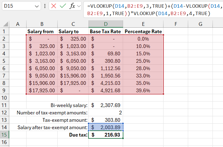
The image below illustrates the method of calculating the tax amount. The tax rate table does not contain all possible options, but only certain boundary limits. First, you need to determine in which tax rate range the employee’s salary falls. Then, use the information from the nearest found value for tax calculations:
=VLOOKUP(D14,B2:E9,3,TRUE)+(D14-VLOOKUP(D14,B2:E9,1,TRUE))*VLOOKUP(D14,B2:E9,4,TRUE)

The formula uses three VLOOKUP functions to read three values from the table. In the last argument of each function, the logical value TRUE is used. This means that an approximate value needs to be found, not an exact match.
For any Excel lookup function like VLOOKUP, HLOOKUP, or MATCH with TRUE in the third argument to return the correct result, the data in the searched column (in this example, it’s the range of cells B2:B9) must be sorted in ascending order. The VLOOKUP function checks all values sequentially and stops searching if the next value is greater than the search value. This is why the initial range must be sorted in ascending order. This way, the largest value that is still less than the search value is found.
Attention! Excel’s lookup functions for approximate matching do not find the closest possible value. Instead, they return the largest number that is smaller than the search value, even if the next checked value is much closer to the search value.
Attention! If the data in the column being searched is not sorted in ascending order, the lookup function will return an incorrect result (which is worse than an error!) instead of an error. Lookup functions designed for approximate matching use a binary search method. This method begins by checking the middle of the column and determines whether the search value is in the upper or lower half. Once the correct half is found, it is divided again, and the process repeats until a result is found.
Thus, a binary search on unsorted data ranges can often lead to the lookup function selecting the wrong half of the column and returning an incorrect result (without an error code).
In the above example, the VLOOKUP function will stop searching at the second row of the column because the number 1023 is the largest number less than the search value of 2003.89. The formula can be broken down into three steps, which perform the following operations:
- The first VLOOKUP function returns the base tax rate from the third column of the table, which is the number 69.80.
- The next VLOOKUP function searches for the same approximate value for 2003.89, but from the first column “Salary from.” The found approximate value is then subtracted from the search value.
- The third VLOOKUP function returns the percentage rate from the fourth column of the table. The rate is multiplied by the net salary (after all deductions), and the result is added to the base rate.
Once all VLOOKUP functions return their results, the following arithmetic calculations are performed:
=69.80+(2003.89-1023.00)*15.0%
Searching for data with approximate matching is significantly faster than with exact matching. In an exact match search, the lookup function must check each cell in the searched column one by one. If you are sure that the source data in the searched column is sorted in ascending order, you can speed up the exact search by specifying TRUE in the third argument. In the case of approximate matching, the exact match with the search value will always be found, provided it actually exists in the list and the list is sorted in ascending order.
Example Formula for Approximate Search with INDEX and MATCH in Excel
Any lookup function can be replaced with a formula that combines the INDEX and MATCH functions. The last argument of the MATCH function allows switching between approximate and exact search, similar to VLOOKUP and HLOOKUP. However, the advantage of the MATCH function is that it can perform an approximate search with data sorted in descending order.
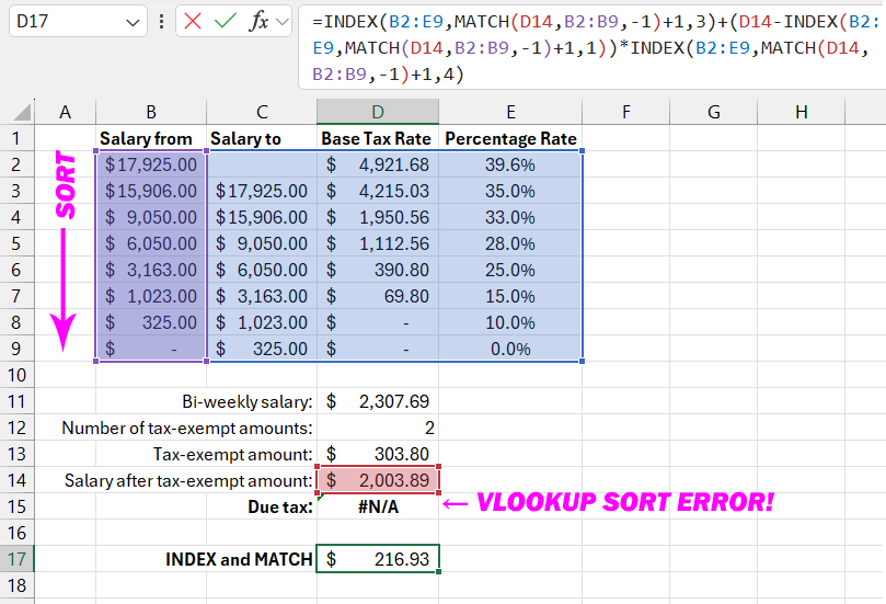
The image below shows the same tax rate table, but sorted in descending order. The new formula in the cell … uses the INDEX and MATCH functions and returns the correct result:
=INDEX(B2:E9,MATCH(D14,B2:B9,-1)+1,3)+(D14-INDEX(B2:E9,MATCH(D14,B2:B9,-1)+1,1))*INDEX(B2:E9,MATCH(D14,B2:B9,-1)+1,4)

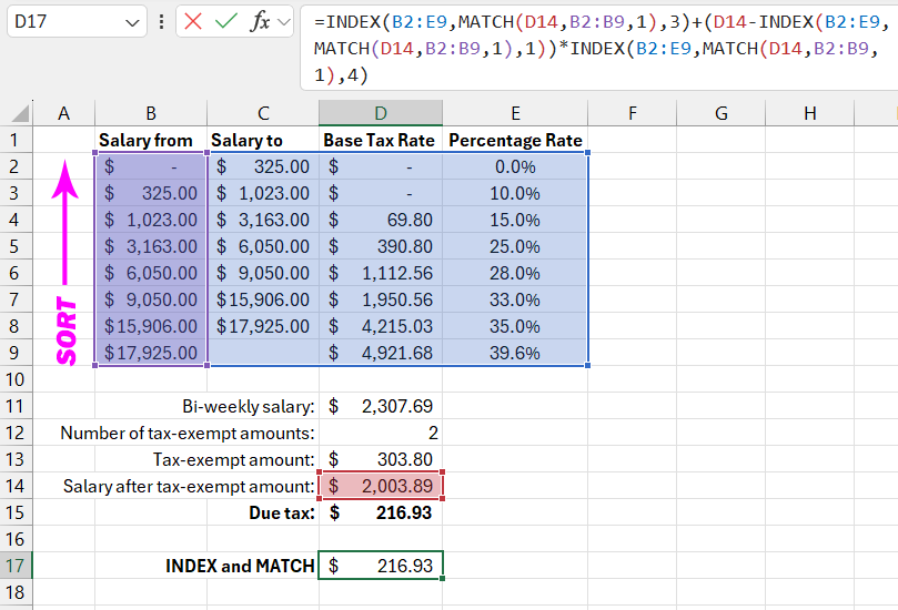
When changing the sort order to ascending, remember to adjust the arguments in the INDEX and MATCH functions.
=INDEX(B2:E9,MATCH(D14,B2:B9,1),3)+(D14-INDEX(B2:E9,MATCH(D14,B2:B9,1),1))*INDEX(B2:E9,MATCH(D14,B2:B9,1),4)

Download an example of formulas for approximate search in Excel 
The old VLOOKUP formula in this case returns the #N/A error instead of the final result in cell D15. This happens because VLOOKUP starts searching from the middle of the column and determines that the search value is smaller. Therefore, it analyzes only the upper half of the column. Since the values are sorted in descending order, no value smaller than the search value can be found in the upper half.
Meanwhile, the new formula in cell D17 returns the correct final result.
Unlike other lookup functions, the last argument of the MATCH function can be a negative number, specifically one of three options: -1, 0, 1:
- A negative value of -1 is used when working with data sorted in descending order. The function returns the smallest value that is greater than the search value. You cannot use -1 in the third argument for lookup functions like VLOOKUP and HLOOKUP, as there is no such mode of operation for these functions.
- The value 0 is used for searching unsorted data to find an exact match. The behavior of the MATCH function with 0 in the third argument is similar to the behavior of VLOOKUP and HLOOKUP with FALSE or 0 in the third argument.
- The value 1 applies to data sorted in ascending order. In this case, the function returns the largest value that is less than the search value. A positive number 1 in the third argument of the MATCH function works similarly to TRUE or 1 for VLOOKUP and HLOOKUP in the same argument.
Since the MATCH function with -1 as the last argument searches for a value greater than the search value, you should add +1 to the result to get the correct row number for the INDEX function.
