How to Use Array Formulas in Excel Table with an Example

How do you know if a given formula is an array formula? What does it even mean?

When creating a formula (or function), it is neither an array formula nor a regular formula by itself. You define how Excel should interpret the formula you enter. The fact that a formula is an array formula is not so much a feature of the formula itself, but rather how Excel processes it. Confirming a formula with the "Ctrl + Shift + Enter" key combination tells Excel to treat it as an array of calculations. It is then used as a function argument and returns a table (data array) as the result of the calculations.



Examples of Array Formulas and the Difference from Regular Formulas in Excel

Some Excel functions, by default, take a range of cells (an array) as an argument and return a single value. Great examples are the SUM, COUNTIF, AVERAGE functions, etc. For these functions, it doesn’t matter whether you enter them as array functions or not. They handle tables and will work correctly in any situation. These are the "Excel survivors," so to speak.

Fortunately, there are other functions that work differently, depending on whether or not they are treated as "array functions." A perfect example is the IF function.

When Is a Formula an Array Formula and When Is It Regular?

First, let's define what a regular array of values looks like in Excel. These are values enclosed in curly braces and separated by semicolons. For example:

{23;-32;15;7} – this is the syntax of a value array in Excel. It can be used in function arguments.

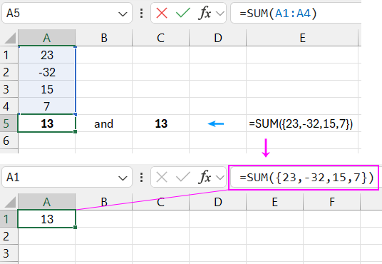
The range of cells A1:A4 is also an array of values in Excel, and can also be used in function arguments. For example, compare the results of two formulas: =SUM(A1:A4) and =SUM({23;-32;15;7}) – they are identical:

Visually, an array formula is also enclosed in curly braces, but they should not be entered manually, only using the Ctrl + Shift + Enter key combination. If you manually enter the curly braces, the formula will not work as an array – this will be a syntax error in Excel.

An array formula (entered using Ctrl + Shift + Enter) will be used whenever you want a function that usually works with individual values (cells) to behave differently and accept an array of values (a table) as both an argument and result. Let’s return to the previously mentioned IF function. As an argument, it takes a logical value of TRUE or FALSE. In the classic form:

=IF($A$1>0,"greater","less")

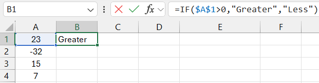
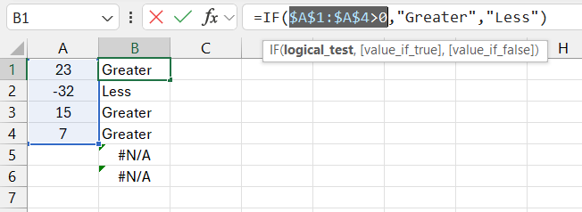
If the value in cell A1 is greater than zero, the function will receive the argument TRUE and return the text string "greater." However, if you wanted to check several cells at once and pass the result of that check to another function, you would need to use the above formula as an array formula. To do this, press Ctrl + Shift + Enter instead of the usual Enter:

{=IF($A$1:$A$4>0,"greater","less")}

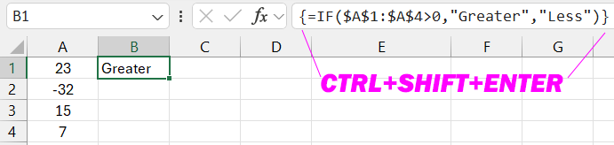
The function takes the entire range $A$1:$A$4 as an argument. As a result of checking each cell in the range, a table of values is created in the computer's memory. The table can be schematically represented as follows:

And these values look like this in the array:

{TRUE;FALSE;TRUE;TRUE}

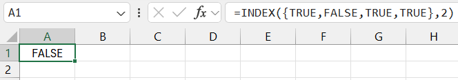
For example, to read this array and retrieve the second value, you can use the function:

=INDEX({TRUE;FALSE;TRUE;TRUE},2)

This is the same as:

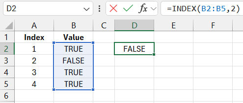
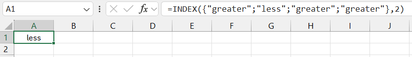
Next, another table is created, with values directly dependent on the values in the first table. If an element in the first array is TRUE, it will take the value "greater" in the second array. If it is FALSE, the element in the second table will take the value "less." After this operation, the first table is deleted from the computer's memory, and the function returns the array {"greater", "less", "greater", "greater"}. The second table can be schematically represented as follows:

You can also read it with the function:

=INDEX({"greater";"less";"greater";"greater"},2)

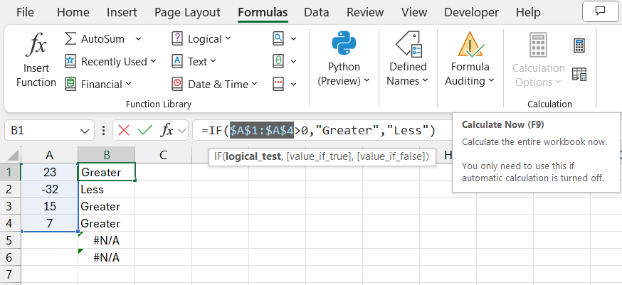
In the example with the IF function, the array formula was entered into only one cell, so we got just one value corresponding to the first value in the result table. However, you can enter the array formula into a range of cells to see all the array values. To do this, select a range of multiple cells, press F2 (or re-enter the formula manually), and press Ctrl + Shift + Enter.

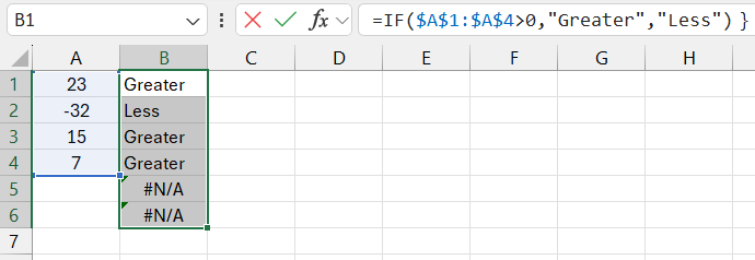
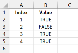
In the example below, you can see that the result table contains exactly four elements, as mentioned earlier.

Examples of Using Array Formulas in Excel

This all sounds good, but some questions arise: "Why do I need an array formula?" or "How and where do I use an array formula?" and "How is it better than a regular formula?"

Of course, an array returned by the IF function can be passed on for further "processing" as an argument to another function.

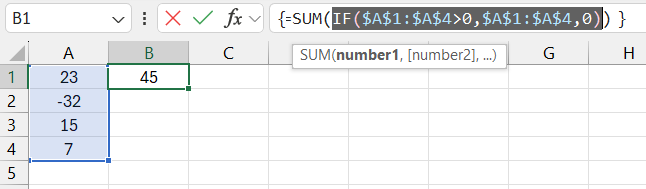
Example: Let's imagine you want to find the sum of the cells B7:B10, but only those that are greater than zero. Sure, you could use the SUMIF function, but in our example, we want to do this using only an array formula. When summing the values of the cells in our range, we need to somehow eliminate the value "-32". The SUM function must be provided with an array that contains only values greater than zero. Wherever the value is less than zero, we replace it with zero, which of course will not affect the result. As you already know, you can obtain a temporary table with the appropriate values using the IF function. Ultimately, the corresponding formula will look like this:

=SUM(IF($A$1:$A$4>0,$A$1:$A$4,0))

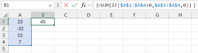
Enter the formula and don't forget to confirm the entry by pressing the CTRL+SHIFT+Enter key combination. As a result of checking each cell in the range $A$1:$A$4 (whether the value is greater than zero), a memory array {TRUE; FALSE; TRUE; TRUE} is created. Then, another table is created. If an element in the first array is TRUE, the corresponding value from the range will be displayed in the second table. If it is FALSE, the element in the second table will take the value 0. After this operation, the first table is deleted from the computer’s memory, and ultimately the IF function returns an array {23; 0; 15; 7}. This table is then passed as an argument to the SUM function =SUM({23; 0; 15; 7}), which, according to its purpose, returns the sum of all the elements in the table. In our example, the sum equals 45. Finally, observe what happens if you instruct Excel to process the above formula as a non-array formula. In new versions of Excel, starting from 2019, dynamic ranges appeared and now array formulas are used much less frequently.

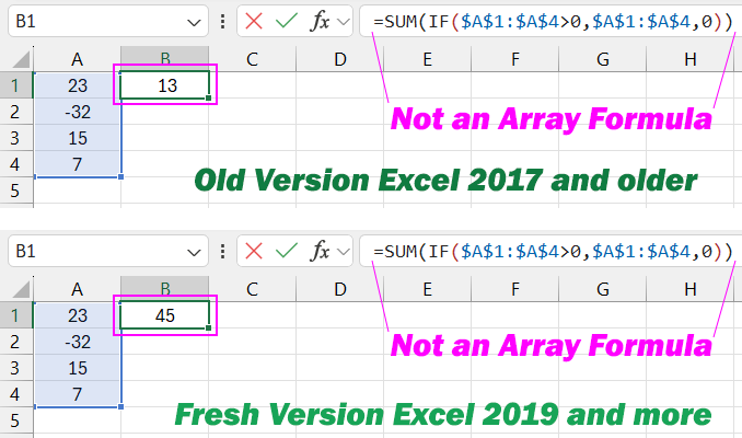
None of the tables described above will be created in this case. Only one cell from the range will be checked (the cell in the same row as the function). In our case, 15>0 means that the first argument the IF function will receive is the logical value TRUE. Then, the ENTIRE range A1:A4 will be passed to the SUM function, resulting in a sum of 13 (23-32+15+7). If the value in the cell was less than zero, the IF function would return FALSE, and only zero would be passed to the SUM function, resulting in a sum of zero.

How to Distinguish an Array Formula from a Regular Formula

When you press CTRL+SHIFT+Enter to confirm entry, curly braces will appear around the formula in the formula bar, indicating that it is an array formula. But what if you're not sure whether to use an array formula during creation?

Correctly identifying when to press CTRL+SHIFT+Enter versus simply pressing Enter depends entirely on understanding how arrays work in formulas. Once you grasp this, you'll know when a formula should be confirmed with CTRL+SHIFT+Enter.

Of course, a formula not confirmed as an array formula may still return SOME result (as you've just seen for yourself). However, if you can read and understand the formula's mechanism, you'll notice that the result is INCORRECT. That's why to ensure the formula works correctly, you need to confirm it with "Ctrl+Shift+Enter." As with everything, understanding and using array formulas requires practice. Still, it’s worth spending some time mastering it, as array formulas allow you to solve many problems that may initially seem unsolvable.

Examples of Calculations and Analysis of Array Formulas

How can you view and check the intermediate results of a calculation, such as the contents of arrays created in memory and used for subsequent operations? It's not difficult! Example 1:

Select the cell with the formula, and then in the formula bar, highlight the reference to the cell range in the first function argument:

Press F9 (or "Recalculate" in the top-right corner of the "Formulas" menu), and you'll see (in the formula bar) the values of the arguments used for the calculations, as shown below:

- The notation using colons means that we are dealing with vertical (column) array elements, and horizontal (row) elements are separated by the standard symbol - ";" (semicolon).

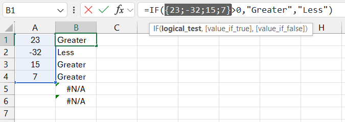
Example 2: Again, go to the cell with the array formula, but this time select the first argument of the function entirely, including the comparison sign ">" and the criterion "0".

Press the F9 button, and you’ll get the array of calculation results, as shown below:

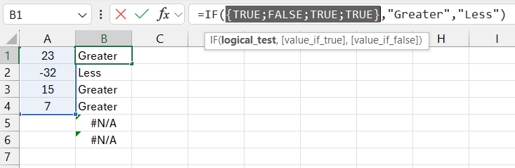
That is, the array created in the computer's memory:

{TRUE:FALSE:TRUE:TRUE}

Example 3: Select the cell with the array formula where the SUM function includes the IF function. Then in the formula bar, select the entire argument of the SUM function (including the IF function):

Press F9 and you'll see the final array of calculation results used for summing, as shown below:

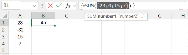
That is, the array created in the computer’s memory:

{23\0\15\7}

Example 4: Simply go to the cell with the formula in B1 and select the "FORMULAS"-"Formula Auditing"-"Evaluate Formula" tool:

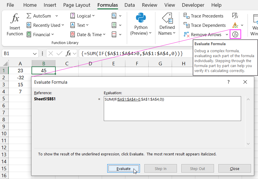
Then click the "Evaluate" button:

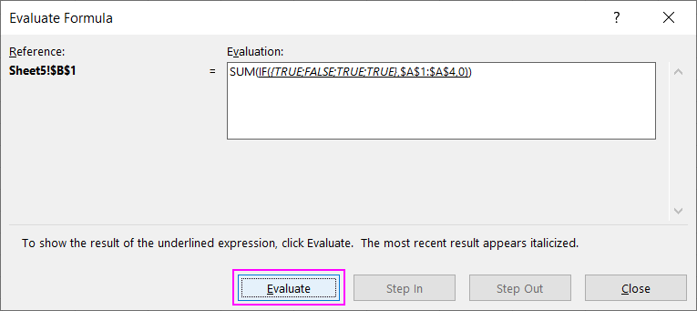
As a result, the reference to the cell range in the argument of the nested IF function was broken down into an array of values. Click "Evaluate" again:

Download examples of using array formulas in Excel spreadsheets

We have now obtained the array of values for the SUM function, just as in Example 3.

Read also: Working with Excel Function Arrays.

Often, inexperienced Excel users complain that a formula isn’t working. In the end, as you can guess, the array formula was entered as a regular one (simply by pressing Enter). The issue isn’t just the misunderstanding, but that these users begin to wonder how to avoid such mistakes. That’s why it’s important to fully understand how array formulas work so that such questions don’t arise in the future.