How to use HLOOKUP formula to extract data by rows in Excel

If the data is organized so that the value to be found is in the first row instead of the first column, you need to perform a search by rows, not columns. Excel has a function called HLOOKUP—specifically designed for horizontal lookup across rows in tables.



HLOOKUP Formula and Row Lookup in Excel for Beginners

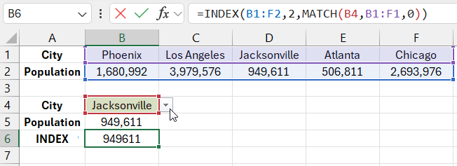
Below is a picture of a table with population data for the largest cities in Russia. After the user selects a city from the dropdown list, the population corresponding to the selected city is automatically filled in the cell below. The formula is:

=HLOOKUP(B4,B1:F2,2,FALSE)

The HLOOKUP function has the same arguments in its syntax as VLOOKUP. The key difference is that HLOOKUP searches the specified range in the first row, not the first column, like VLOOKUP. If the value is found, it returns the content of the cell from the second row and corresponding column.

INDEX and MATCH Formula for Horizontal Row Lookup

The HLOOKUP and VLOOKUP functions are very similar. Both can be replaced with a combination of the INDEX and MATCH functions:

=INDEX(B1:F2,2,MATCH(B4,B1:F1,0))

Download the Example: How to Use the HLOOKUP Formula in Excel

In this example, the row number in the INDEX function is predefined by the user and is fixed—it’s the number 2. The MATCH function automatically determines the value for the third argument of the INDEX function. MATCH can only search through one row or one column of cells. When it finds the content matching the lookup value, the function returns its position in the row.