Using EXACT Formula for Exact Text Matching in Excel Table
Functions like VLOOKUP and other lookup functions in Excel do not differentiate between most characters in the values they search. For example, for values like "Payment" and "payment," VLOOKUP would return the same result. If case sensitivity is important, use the EXACT function.
How to Perform Exact Text Search in an Excel Column
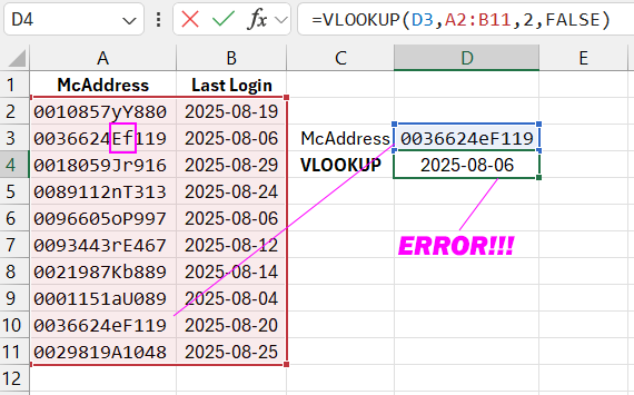
Below is an image showing a list of MAC addresses of network cards and the dates of the last login to the admin panel. The MAC addresses in rows 3 and 10 look identical except for two characters in the middle (Ef and eF). Suppose we need to find the MAC address with case sensitivity. The formula:

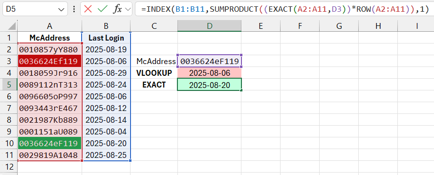
The image above shows the results of two formulas. The first formula uses VLOOKUP in cell D4: =VLOOKUP(D3,A2:B11,2,FALSE), and the second uses EXACT. Although cell D3 contains the MAC address from row 10, the VLOOKUP function returns the value from row 3.
The second formula, which uses the EXACT function, returns the correct result:
=INDEX(B1:B11,SUMPRODUCT((EXACT(A2:A11,D3))*ROW(A2:A11)),1)

Now, you will learn how to use the SUMPRODUCT and ROW functions to determine the row number for the INDEX function by composing a simple formula.
The EXACT function contains 2 arguments and compares their values against each other. The result is a logical TRUE if both arguments are identical (case-sensitive).
How the Formula Works for Exact Matching When Searching Columns
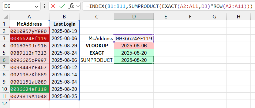
The EXACT function, when used inside the SUMPRODUCT function or as an array formula, can compare ranges of text values with other types of values.
=INDEX(B1:B11,SUMPRODUCT(EXACT(A2:A11,D3)*ROW(A2:A11)))

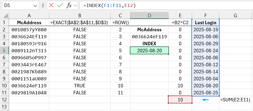
The result will be an array of logical TRUE and FALSE values. In this example, the EXACT function returns TRUE only when comparing the values in cells A10 and D3. When performing arithmetic operations inside the multiplication function, TRUE values are replaced by 1, and FALSE values are replaced by 0. As a result, the SUMPRODUCT function sums all the values and returns the number 10 for the INDEX function. All other values are FALSE=0, and anything multiplied by zero is 0. The principle of the SUMPRODUCT function can be schematically represented as follows:

Download an example of how to use the EXACT formula for searching in Excel 
The number 10 returned by the SUMPRODUCT function is used as the row number argument in the INDEX function, which returns the content of the adjacent cell to the right, B10, on the 10th row of the range B1:B11.
