Calculation of credit in Excel and the formula of monthly payments

Excel - is the versatile analytical and computational tool that is often used by lenders (banks, investors, etc.) and borrowers (businessmen, companies, private persons, etc.).

Quickly navigate in the intricate formulas, calculate to interest, payouts, overpayment to allow Microsoft Excel program functions.



How to calculate credit payments in Excel

Monthly payments depend on the loan repayment scheme. There are annuity and differentiated payments:

1. The annuity assumes that the client makes each month the same amount.
2. When the differentiated scheme of repayment of debt before the financial organization interest is charged on the balance of the loan amount. Therefore, the monthly payments will be reduced.

Increasingly used annuity: it`s more profitable for the bank, and it is more convenient for the majority of customers.

The calculation of annuity payments on the loan in Excel

The monthly annuity payment is calculated as follows:

S = C * V

where:

• S – sum, is the payment amount on the loan;
• C – coefficient, is the annuity payment rate;
• V – is the value of the loan.

The annuity factor Formula:

С = (i * (1 + i) ^ n) / ((1 + i) ^ n-1)

• where is i – the interest rate for the month, the result of dividing the annual rate by 12;
• n – is the loan term in months.

There is a special feature in Excel which said to the annuity payments. This is: =PMT().

1. Fill in the input data for calculating the monthly payments on the credit. This is loan amount, interest and term.
2. To make the repayment schedule. It`s empty till.
3. In the first cell of the column «Credit payments», introduced the formula of the calculating the loan annuity payments in Excel: =PMT($B$3/12,$B$4,$B$2). To fix the cells, are used to the absolute links. In the formula may be administered directly to the numbers and not the reference cell data. Then it will have the following form: =PMT(18%/12,36,100000).

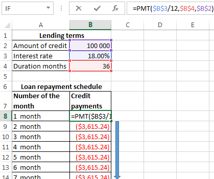
The cells turned into red, because we'll give these money to the bank and to lose the money.



The calculation of payments in Excel for the differentiated scheme of repayment

The differentiated payment method implies that:

• the principal amount is distributed over the period of payment in the equal installments;
• the loan interest accrued on the balance.

The formula for the calculating to the differential payment:

DP = NEO / (PP + PS * NEO)

where:

• DP – is the monthly payment on the loan;
• NEO – is the loan balance;
• PP – the number of remaining until the end of the repayment period;
• PS – is the interest rate per month (the annual rate divided by 12).

Draw up the schedule for repayment of the previous loan on the differentiated scheme.

The input dates are the same:

Lending terms
Amount of credit	$100 000
Interest rate	18%
Duration months	36

To make the schedule of repayment of the loan:

Number of the month	Balance receivable on the loan	Payment of interest	Payment of principal	Final payment
1 month

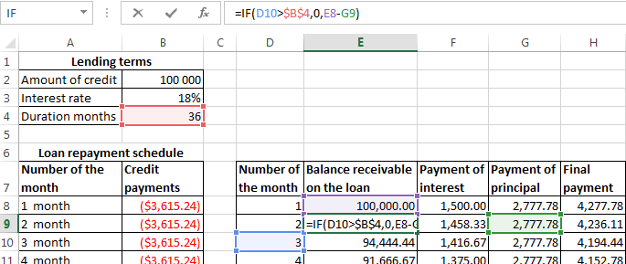
Balance receivable on the loan: in the first month it is equal to the entire amount =$B$2. In the second one and in the subsequent ones - calculated by the formula: =IF(D10>$B$4,0,E8-G9). Where is:

• D10 – the number of the current period;
• $B$4 – is the term of the loan;
• E8 – is the balance of the loan in the previous period;
• G9 - is the principal debt in the previous period.

Payment of interest: the balance of the loan in the current period multiplied by the monthly interest rate / 12 months: =E9*($B$3/12).

Payment of principal: the amount of the loan divided by the period: =IF(D9<=$B$4,$B$2/$B$4,0).

Final payment: the sum of «the interest» and «the main debt» in the current period: =F8+G8.

We substitute to the formulas in the corresponding columns. Copy them to the entire table.

To compare the overpayment on the annuity and the differentiated scheme of the repayment on credit:

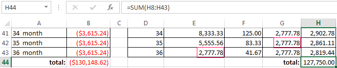
The red figure – is the annuity (was taken 100 000 rubles), the black one – is the differentiated way.

Interest calculation formula for loans in Excel

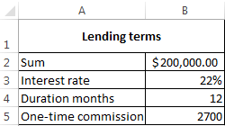
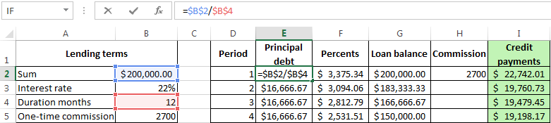
The calculation of interest on the loan in Excel and calculate the effective interest rate, with the following information on the bank offers credit:

We carry out interest calculation on loan and calculate the effective interest rate with the following information on the bank offers credit.

Fill in the table type:

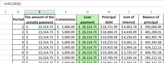
The commission is taken monthly from the whole sum. The total loan payment - this is the annuity payment plus the commission. The sum of the main debt and the sum of interest – there are components parts of the annuity payment.

The principal amount = the annuity payment – the interest.

The sum of interest = the remaining debt * the monthly interest rate.

The balance of principal = the residue of the previous period – the sum of the principal debt in the previous period.

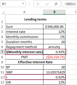
Based on the table of monthly payments, calculate the effective interest rate:

• took the credit 500 000 rubles;
• returned to the bank - 684 881. 67 rubles (the sum of all payments on the loan);
• the overpayment was 184 881. 67 rubles;
• the interest rate - 184 881 67/500 000 * 100, or 37%.
• the harmless commission of 1% was cost for the borrower so expensive.

The effective interest rate of the loan without the commission will be 13%. The counting is carried out in the same way.

The calculation of effective interest rate in Excel

According to the law about the consumer credit for the calculation of the effective interest rate now is applied the new formula. EIR (Effective Interest Rate) is defined in percentage of up to the third decimal place according to the following formula:

• EIR = i * CHBP * 100;
• where is i - the interest rate of the base period;
• NBP - the number of base periods in a calendar year.

Take for example the following dates on the loan:

For calculating of the effective interest rate is necessary to make a payment schedule (see the order above).

It is necessary to determine the base period (BP). The law states that this is the standard time interval, which is found in most of the repayment schedule. Example BP = 28 days.

Then we find NBP: 365/28 = 13.

Now you can find the interest rate of the base period:

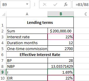
We have all the necessary dates - substitute them in the EIR formula: =B9*B8

To obtain the percentages in Excel, you do not need to multiple by 100. It is enough to set for the cell with the result to the percentage format.

EIR for the new formula is coincided with the annual interest rate on the loan.

Download credit calculator in Excel

Thus, for calculating the annuity payments on the loan is used the simplest function PLT. As you can see, the differentiated way of repayment is a bit more complicated.