Time series analysis and forecasting in Excel with examples
The analysis of time series allows studying the indicators in time. Time series are numerical values of a statistical indicator arranged in chronological order.
Such data are widespread in the most diverse spheres of human activity: daily stock prices, exchange rates, quarterly, annual sales, production, etc. A typical time series in meteorology, for example, is monthly rainfall.
Time series in Excel
If you capture the values of some process at certain intervals, you get the elements of the time series. Their variability is divided into regular and random components. As a rule, regular changes in the members of the series are predictable.
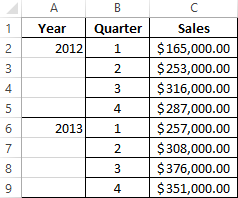
We will analyze time series in Excel. Example: a sales network analyzes data on sales of goods by stores located in cities with a population of fewer than 50,000 people. The period is for 2012-2015. The task is to identify the main development trend.
Enter the sales data in the Excel spreadsheet:
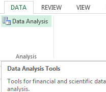
On the «DATA» tab click the «Data Analysis» button. Go to the menu if it is not visible. «Excel Options» – «Add-Ins». Click at the bottom «Go» to «Add-Ins Excel» and select « Data Analysis ».
The connection of the « Data Analysis » add-in is described here in detail.
The button we need appears on the band.
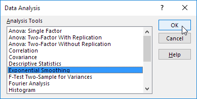
Select «Exponential Smoothing» from the proposed list of tools for statistical analysis. This alignment method is suitable for our dynamic series, the values of which fluctuate strongly.
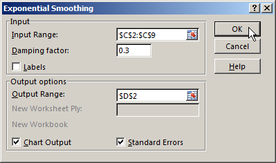
We fill the dialog box. The input interval is the range of sales values. The damping factor is the coefficient of exponential smoothing (default is 0.3). Output interval –is a reference to the upper left cell of the output range. The program will place the smoothed levels here and the will define size independently. We tick the «Chart Output», «Standard Errors».
Close the dialog box by clicking OK. Results of the analysis:
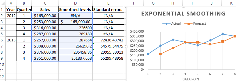
Excel uses next formula to calculate the standard errors: = SQRT(SUMXMY2('Actual value range'; 'range of forecast values') / 'size of the smoothing window'). For example, = SQRT(SUMXMY2:(C3:C5;D3:D5)/3).
Forecasting the time series in Excel
We will compose the forecast of sales using the data from the previous example.
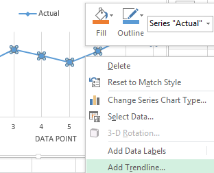
We will add a trend line (the right button on the chart - «Add Trend line») on the chart which shows the actual product sales volume.
Configure the parameters of the trend line:
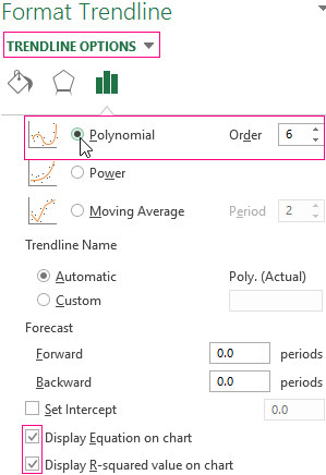
We choose a polynomial trend that minimizes the error of the forecast model.
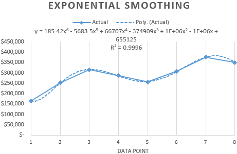
R2 = 0.9567 which means that this ratio explains 95.67% of changes in sales in process of time.
The trend equation is a model of the formula for calculating the forecast values.
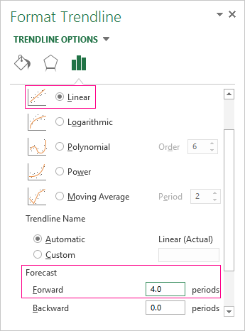
Most authors recommend using a linear trend line for forecasting sales. You need to set the number of periods in the parameters to see the forecast on the chart.
We get a fairly optimistic result:
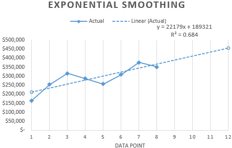
After all, there is the exponential dependence in our example. Therefore, there are more errors and inaccuracies when building a linear trend.
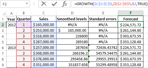
You can also use the function GROWTH to predict the exponential dependence in Excel.
For linear dependence, use the TREND function.
You cannot use any one method when making forecasts: the probability of large deviations and inaccuracies is large.
