How to Create a Step Chart in Excel Download Template

A step chart in Excel is an excellent tool for analyzing discrete changes over a specific period. If you want to represent changes, such as percentage rates, tax rates, or specific stock prices, this chart will undoubtedly serve its purpose. Since Excel doesn't offer a step chart in its default chart templates, today we'll learn how to easily create one ourselves.

 

What Is a Step Chart, and What Are Its Advantages?

A step chart in Excel is essentially a line chart consisting only of vertical and horizontal lines that, when connected, resemble stairs. The vertical lines illustrate the magnitude of resulting changes, while the horizontal lines represent the durations of these changes. Let's check how the original data for a step chart differs from a line chart and explore the advantages of a step chart over a line chart.

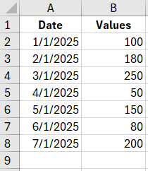
Start by filling in a small table with the original data:

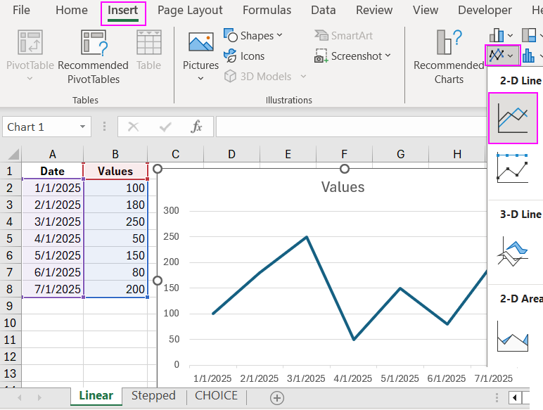
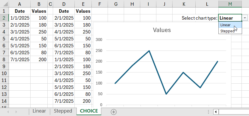
Now, let's create a regular line chart based on this table. Select the range A2:B8 and choose the tool: "INSERT" - "Charts" - "Insert Chart." The result will be as follows:

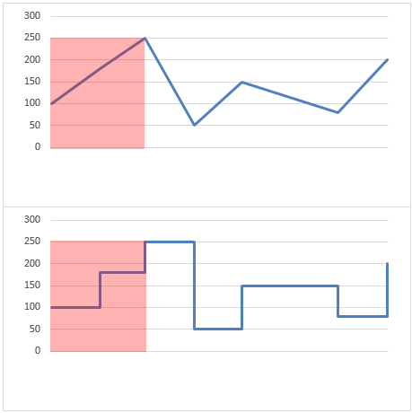
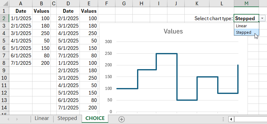
Now, compare it with our future step chart. As seen in the image below, the step chart can display the actual number of changes for a specific part of the total time period, unlike the linear chart:

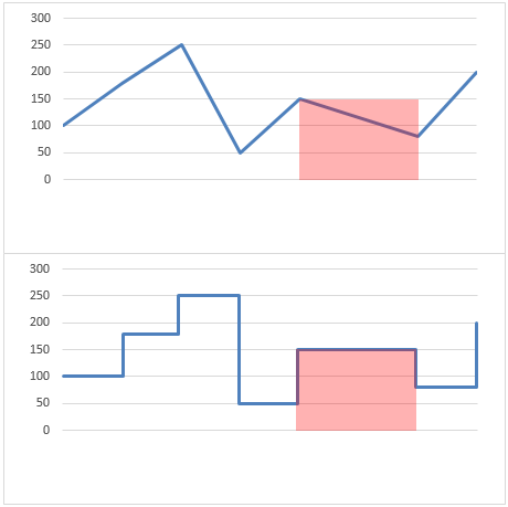
Additionally, the step chart shows us the duration of changes, not just the trend:

In this example, we'll create a switcher between the step and line charts for convenient comparison. As a result, we'll have two visual reports for a more detailed analysis of the data.

How to Create a Step Chart in Excel

We'll use the same original data. First, copy the range A2:B8 and paste it below in the A9:B15 area:

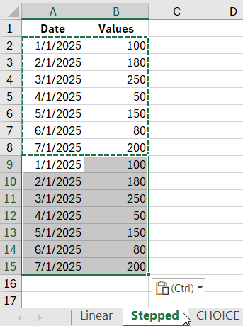
Now, perform the following steps: select the range B2:B15, hover over the selection border, hold the left mouse button, and shift this range down by one cell. Do the same for the range A9:A15. After that, delete the extra rows from the sheet:

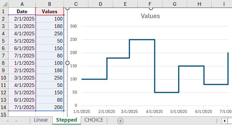
Next, remove rows 9 and 2 from the table. As a result, you'll get a new set of original data for creating a step chart in Excel. Select the range A2:B14 and create a regular line chart based on it. Again, use the tool: "INSERT" - "Charts" - "Insert Chart."

Switching Between Step and Line Charts

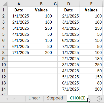
To achieve this, create two tables on a separate Excel sheet named "SELECTION" for the line and step charts:

Also, create a control element for our report for visual analysis. In this example, we'll use a drop-down list. To create a drop-down list in Excel, go to cell M2 and choose the tool: "DATA" - "Data Tools" - "Data Validation":

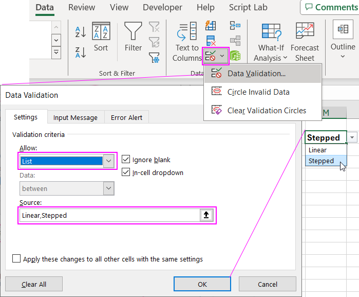
In the "Data Validation" dialog box, on the "Settings" tab, in the "Allow" options, select "List." In the "Source" field, enter the following text: Linear;Step. Now, whenever you change the value in cell M2 using the drop-down list, the references to the series (Y-axis) and categories (X-axis) for the step and line charts will automatically change:

Download Step Chart Template in Excel

In this example, we've shown the quickest way to turn a line chart into a step chart in Excel without complex design formatting. Moreover, you have the flexibility to switch between the two modes for a detailed and general analysis of the history of metric changes.