How to Make Forecast Using Holt Winters Model in Excel

Excel is a versatile tool for various types of analysis, including forecasting. In this example, we'll explore how to use Excel for forecasting using the Holt-Winters model. You can download the finished forecast file at the end of the example.

 

How to build the Holt-Winters model for forecasting in Excel

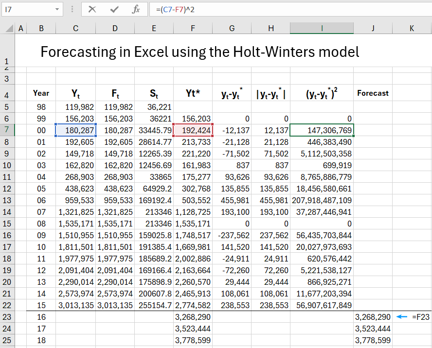
We will build our Holt-Winters forecast model based on statistical data from an airport. Using the model, we'll attempt to predict the number of passengers served in international regulated air traffic from 2016-2018. Our table will have columns indicating: C(Yt) - the number of serviced passengers, D(Ft) - estimate of random variations in the model, E(St) - estimate of the trend for the model, F(Yt*) - expired and actual forecasts, G(yt-yt*);H(|yt-yt*|);I((yt-yt*)2) - calculations needed for MAE, MSE, RMSE indicators, MN - alpha and beta parameters for the model.

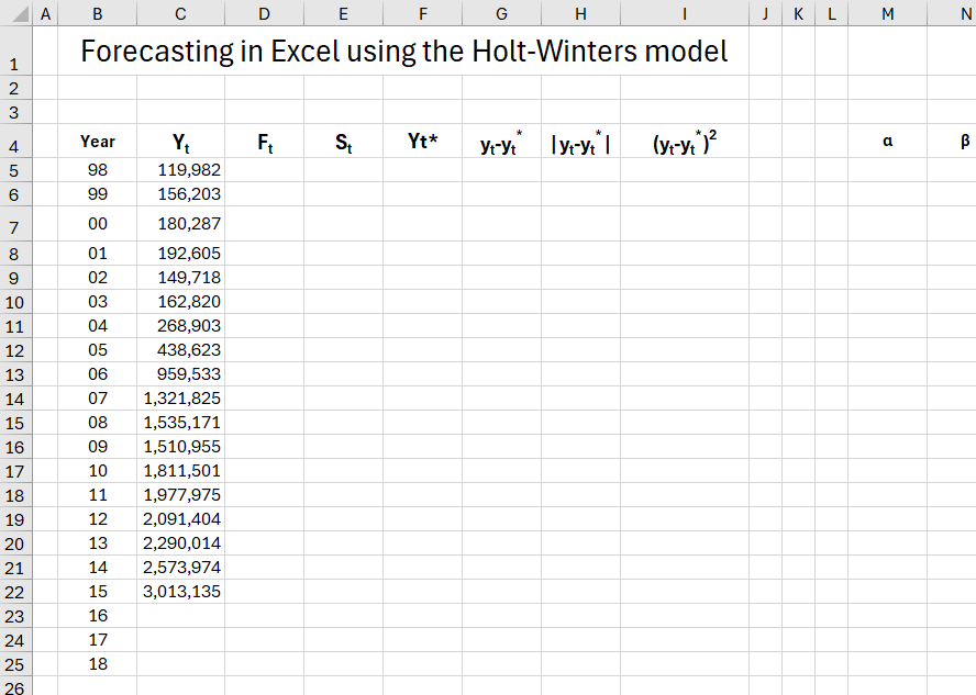
We'll create a forecast considering all the rules of the Holt-Winters model using Excel formulas, and based on the obtained data, we'll create a graph for visual analysis.

Forecasting method using the Holt-Winters model in Excel

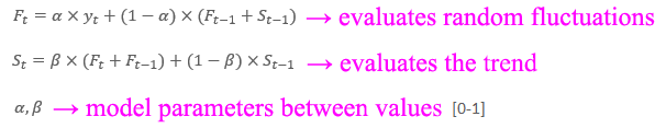
The Holt-Winters model is one of the forecasting methods using exponential smoothing. Smoothing involves creating a weighted moving average, where the weight is determined by the scheme - the older the information about the phenomenon under study, the less its value for the current forecast. To build the model, make the following assumptions and formulas.

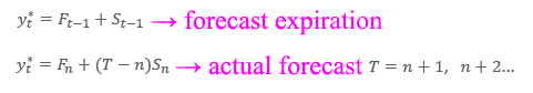
The model calculates forecasts with an expired term, i.e., those related to the period in which the actual value has already been realized, and real forecasts for the period that has not yet occurred.

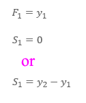
Initial values F1 and S1 are usually:

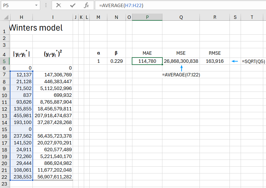
To assess the accuracy of the model's forecasts, we use the so-called actual error of expired forecasts using indicators:

Mean Absolute Error (MAE) - tells us, on average over the forecast period, how much the actual values of the forecasted variable will deviate relative to the absolute value from the forecasts.

Mean Squared Error (MSE) - is the average difference in the square of the deviations between the actual realizations of the forecasted variable and the forecast.

where Yt* - expired forecasts.

Root Mean Square Error (RMSE) - measures how much the deviation of the realization of the forecasted variable from the calculated forecasts.

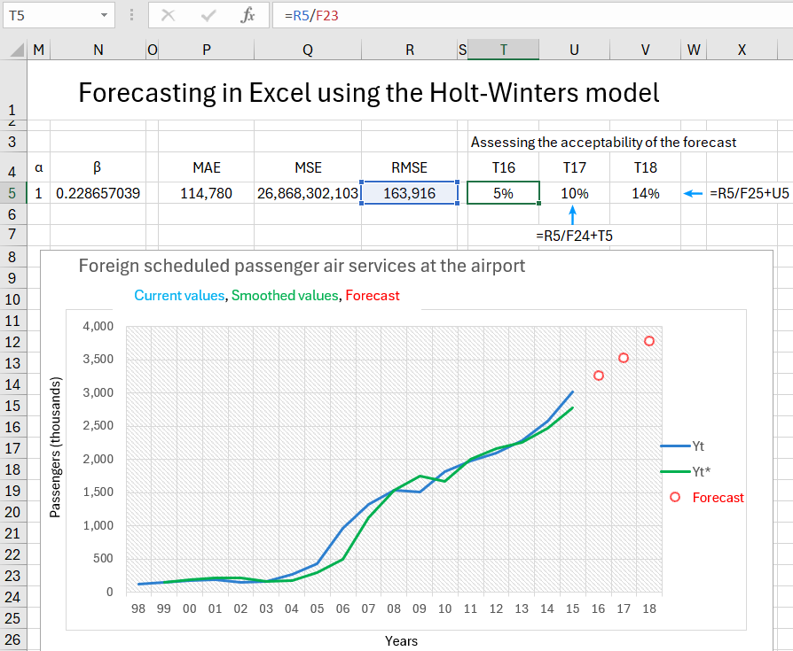
Once the model is created, it can be considered good if the ratio of RMSE to the actual forecasting is less than 10%. However, in practice, the best test for evaluating the effectiveness of the model will be to compare the forecasts it creates with actual values.

Formulas for the Holt-Winters forecast model in Excel

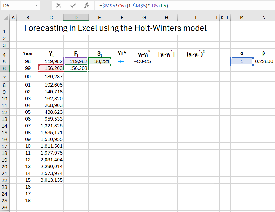
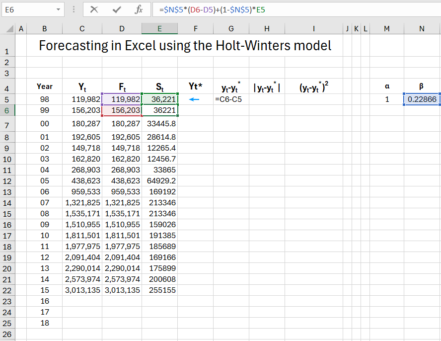
Now, according to the assumptions made earlier, we provide initial values for the parameters F1 and S1. In our case, this will be y1 = F1 and y2-y1 = S1. Next, we enter the alpha and beta parameters, temporarily assuming their values are 0.4 (later we will optimize the data using the Solver's "Goal Seek" tool). Anticipating, let's assume these will be values for α = 1 (cell M5) and for β 0.2286 (cell N5), so you can enter these values right away, whichever is more convenient for you.

Next, we calculate Ft and St simultaneously according to the formulas provided above, dragging the formulas down.

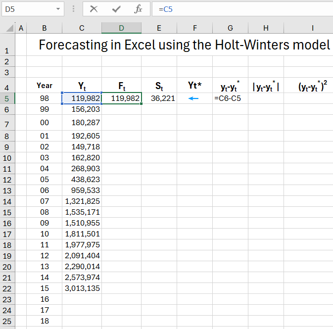
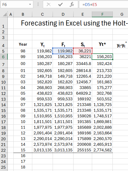
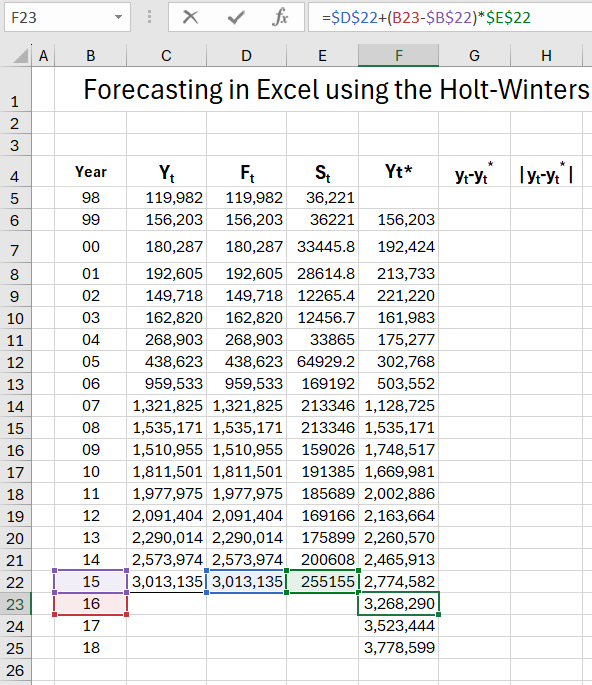
Move on to column F, where using formulas, we calculate that for 1998-2015 forecasts expired, and for 2016-2018, real forecasts.

We fill in columns GI, which will currently be used to calculate the actual error of expired forecasts (to obtain the absolute value in column H, we can use the Excel function =ABS()).

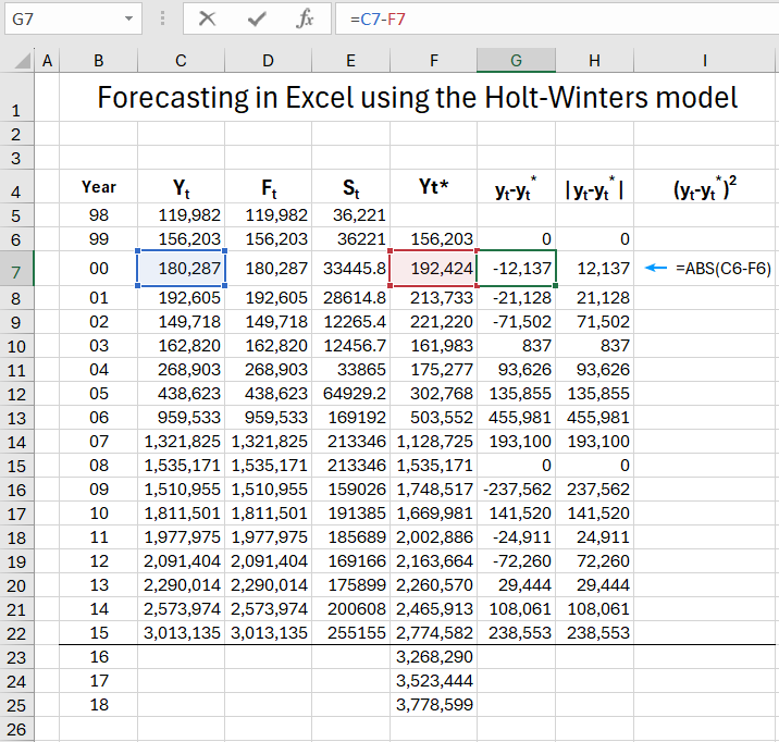
Then, using the =AVERAGE() and =SQRT() functions, we calculate the above-mentioned error indicators MAE, MSE, and RMSE.

After calculating the indicators, we can proceed to optimize the alpha and beta parameters so that the MAE index is as small as possible. To do this, we'll use the "Goal Seek" analytical tool in Excel, available on the "DATA" tab in the "Analysis" group. Set the search solution parameters to minimize the MAE index by changing cells marked as alpha and beta, constrained in the range [0-1].

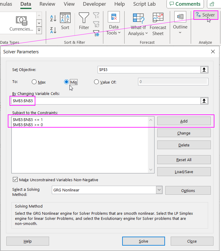
If you can't find the "Analysis" tab and Solver button in the MS Excel application interface, use the instructions for enabling this feature in the settings from this article: How to calculate the optimal log breakdown in Excel.

After clicking the "Solve" button and saving the obtained results, the alpha and beta smoothing parameters should be a = 1 and b = 0.228657122399511. At this stage, we can preliminarily check whether our model can be used as an effective forecasting tool. For this purpose, we calculate the acceptability coefficient of the forecast, determined by the formula RMSE / actual forecast for subsequent periods T16-T18. In our case, for 2016, this is 5%, so the forecast can be considered reliable. Finally, it's worth visualizing the entire analysis on a graph, taking actual values and forecasts as data series.

Download an example of a Holt Winters forecast in Excel

Once we have a forecast, there's nothing left to do but monitor new data to check if the model makes sense in practice. From information available on one of the company's flight information portals, the total number of passengers served in 2017 was over 4.6 million people. Therefore, there's a high probability that the values we forecasted work in practice.