Assigning the mathematical function SUM in Excel example
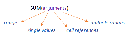
SUM in Excel is a mathematical function used to add up numeric values. Arguments can be single values, cell references, a range, or multiple individual ranges.
Practical work with examples of the SUM function in Excel
How does the SUM function work? Schematically, its syntax is as follows:
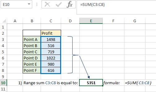
Consider the simplest example of the SUM function. We have a list with a profit for several points of sale and the first task is to calculate the amount of profit for all points. In cell E10 we write the formula. To do this, we select the entire range with values (С3:С8) as arguments:
You can also sum several ranges, for example, we need the sum of the ranges С3:С5 and С6:С8:
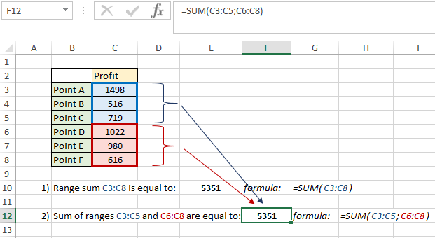
In cell F12, we got the same result as in task 1, which means that the formula worked correctly.
How to use the SUM function with arrays
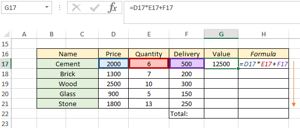
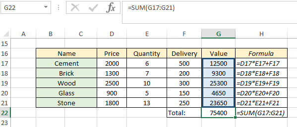
Now let's look at how else we can simplify our tasks with the help of SUM. We have a form with information about building materials, their price, quantity and delivery costs. We need to calculate the total amount of the purchase of goods. Having certain knowledge in EXCEL, the user can perform this task as follows - in cell G17, write the calculation formula "Price * Quantity + Delivery" and copy to the last position:
Then we wrote the SUM function in cell G22, selected the entire range G17:G21 and we have the total cost of buying goods, taking into account the price for the goods, quantity and delivery:
In order to calculate the purchase without resorting to an additional column in which we calculated the cost for an individual product, we use the SUM function and the array formula:
- in cell C24 select the SUM function;
- then select the array D17:D21, put the multiplication symbol;
- select array E17:E21;
- add (+) array F17:F21, close the bracket.
Mandatory moment! After we have filled in the formula, we execute it not through Enter, but by successively pressing the Ctrl + Shift + Enter buttons. If you press Enter, an error will be returned. This time we have curly braces, which means that our formula has summed using array rules:
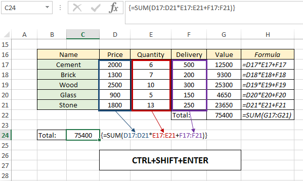
We can compare the results of the two examples (cells G22 and C24) to see if the formulas work the same way.
How to calculate a running total using the SUM function
We have a profit report for every month. After a month, we need to calculate the profit that we have received since the beginning of the year, which means that in March we need to know the amount of profit for January, February, March. In cell D31 we write the formula:
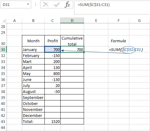
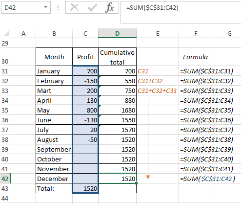
The beginning of the range (C31) will remain unchanged, since we have specified absolute references for this cell. Now we have the same cell C31 at the end of the range, because so far we only need the amount of sales for January. After that, we need to copy the formula to the end of the year. When copying by column, only the end of the range will change. Thus, the calculation of profit for the months from the beginning of the year will take place and we will get the cumulative values:
Summation by selected criteria
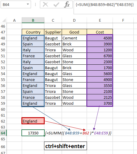
Another example of using the SUM formula will show us how we can calculate the total cost of goods under certain conditions. For example, we have data on the cost of goods of certain suppliers from different countries. We want to know the value of purchased goods from England. In cell B64 we will write the formula:
- select array В48:В59. This array will be searched by the specified condition;
- refer to the cell with the condition ("England", В62);
- put the symbol of multiplication, select the array E48:E59, which contains numeric values;
- successively press the ctrl + shift + enter keys to correctly display the result. Thus, we “tell” the program that an array formula is used.
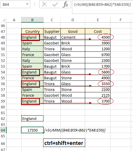
The formula searched the column with countries, found goods from England and calculated their total cost:
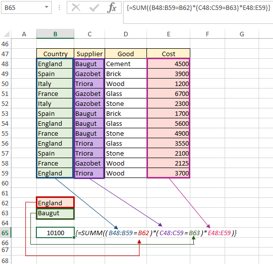
You can use additional conditions. In addition to the criteria for searching by country, we can specify that we want to find the cost of goods from a specific supplier, for example, "Baugut". For convenience, in a separate cell (B63) we indicate the supplier, so that later we can refer to this cell. The algorithm of actions for constructing the formula is exactly the same as in the previous example, just add another array to search for C48:C59 and the desired criterion "Baugut" in cell B63:
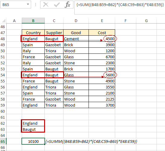
Thanks to this construction, the sum formula not only considers the given values, but also searches by countries, suppliers, or any other criteria that the user wants to specify, and returns the sum of the products found:
How to use the SUM function with other functions
Combining EXCEL functions allows you to expand their functionality. In the following example, we'll look at a simple use of the SUM function along with the OFFSET function in order to understand the logic behind how these functions work together. This time, we need a table that contains information about departments (or functions) and their revenues from 2014 to 2022. Our task is to find the sum of the income of department A and department B in 2014. If you are familiar with the OFFSET function, then you know that its arguments highlight the range of values we need: from cell B71 we take a step two lines up and three columns to the right (the first pair of numbers is -2; 3). Now we "stand" on cell E69. Then we create boundaries for the array whose data we need to sum: 1 row and 2 columns (the second pair of numbers). Thus, we have chosen the E69:F69 range. Now we put the resulting formula into the SUM:
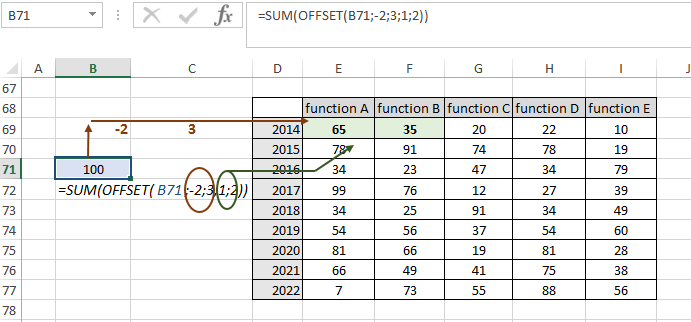
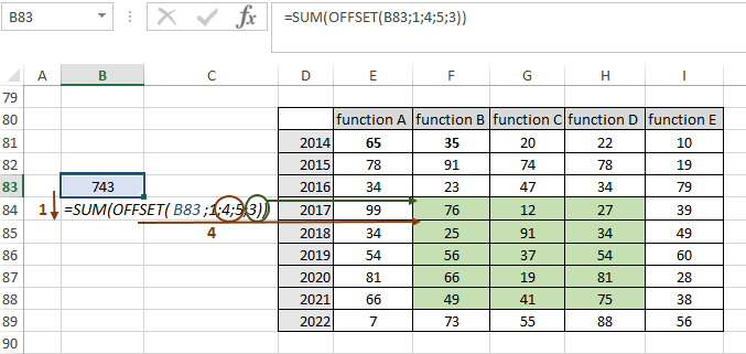
We got a result of 100 (Department A has an income of 65 in 2014, and Department B has 35). Now let's calculate the total income, for example, for departments B, C, D for 2017-2021. We shift our function in the same way:
- argument 1 – cell from which the offset will occur;
- argument 2 – shift down by 1 row;
- argument 3 – shift by 4 columns to the right;
- argument 4 – number of rows in the array (5);
- argument 5 is the number of columns in the array (3).
Validating Input Values with SUM
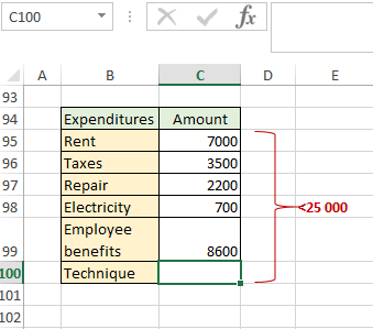
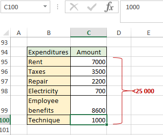
To run this example, we need a cost form and a Data Validation tool. We need to set a limit on the amount of total costs - the amount when adding a new item (cell C100) should not exceed 25,000:
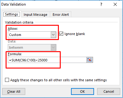
On the "Data" tab - the "Data Tools" group, select the "Data Validation" tool. The Data Validation window will open. In the window that appears, in the validation criteria, select «Custom» from the list. We write our formula:
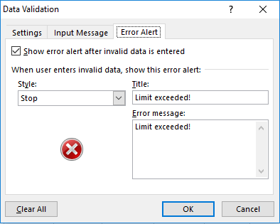
Then go to the "Error Alert" tab and specify the text that we want to see if the condition is not met, for example, "Limit exceeded!":
When we enter a value in cell C100 or change it, data validation will start. As long as the sum of the C95:C100 array is less than 25,000, the check will be successful. We enter the number 1000 and see that nothing happens:
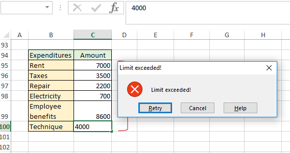
Now we enter the value 4000 and we will see a window with an error that we indicated in the "Error Alert" tab:
 Download Practical Examples of Using the SUM Function in Excel
This happened because the tool recalculated the values for all line items and exceeded the threshold of 25,000.
