Functions CHAR SIGN TYPE in Excel and examples of their formulas
In Excel, it is often necessary to use when calculating values that are tied to symbols, the sign of a number, and the type.
The following functions are used for this:
- CHAR;
- TYPE;
- SIGN.
CHAR function makes it possible to get a character with its given code. The function is used to convert the numeric character codes that are received from other computers into characters of the given computer.
TYPE function determines the data types of the cell, returning the corresponding number.
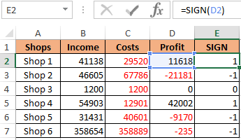
SIGN function returns the sign of a number and returns the value 1 if it is positive, 0 if it is 0, and -1 if it is negative.
Examples of using the CHAR, TYPE and SIGN functions in excel formulas
Example 1. Given a table with character codes: from 65 - to 74:
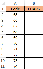
It is necessary with the help of the CHAR to display the characters that correspond to these codes.
To do this, we enter into the cell B2 the following formula:
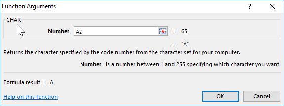
The function argument: Number is the character code.
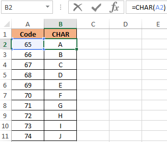
As a result of the calculations we get:
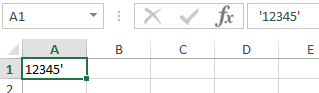
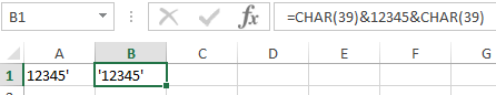
How to use the CHAR in formulas in practice? For example, we need to display a text string in single quotes. For Excel, a single quote as the first character is a special character that converts any cell value to a text data type. Therefore, in the cell itself, the single quote as the first character is not displayed:
To solve this problem, we use the following formula with the function =CHAR(39)
It is also useful to use this function when you need to make a line break in an Excel cell as a formula. And for other similar tasks.
The value 39 in the function argument, you guessed it, is the character code of a single quote.
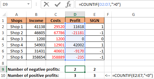
How to count the number of positive and negative numbers in Excel
Example 2. The table contains 3 numbers. Calculate which character has each number: positive (+), negative (-) or 0.
Let's enter the data in the table of the form:
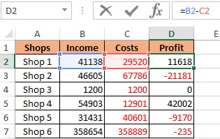
We introduce the formula in cell E2:
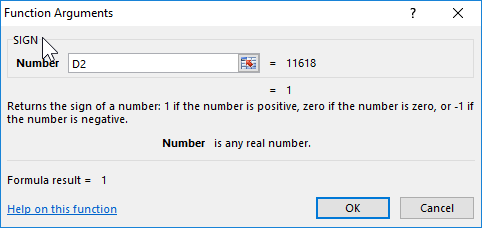
Argument: Number - any real numeric value.
By copying this formula down, we get:
First, we calculate the number of negative and positive numbers in the columns "Profit" and "SIGN":
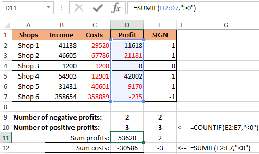
And now we summarize only positive or only negative numbers:
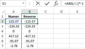
How to make a negative number positive and positive negative? It is very simple to multiply by -1:
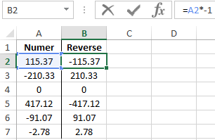
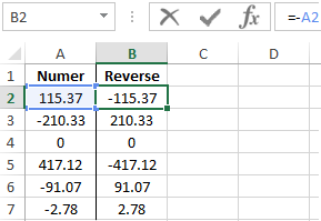
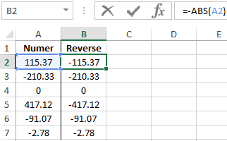
You can even simplify the formula, simply put a subtraction operator sign - minus, before the cell reference:
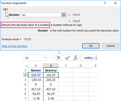
But what if you need to make a number with any sign positive? Then you should use the ABS function. This function returns any number by module:
Now it is not difficult to guess how to make any number with a negative minus sign:
Or so:
Checking what types of cell input data in an Excel spreadsheet
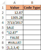
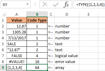
Example 3. Using the TYPE function, display the type of data that is entered in the table:
TYPE function returns the code of the data types that can be entered into an Excel cell:
| Data Value | Type Code |
| number | 1 |
| text | 2 |
| logical value | 4 |
| error value | 16 |
| array | 64 |
We introduce the formula for the calculation in cell B2:
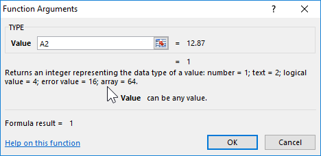
Argument: Value is any valid value.
As a result, we get:
Download examples functions CHAR SIGN TYPE in Excel
Thus, using the TYPE function, you can always check what the Excel cell actually contains. Note that the date is defined by the function as a number. For Excel, any date is a numeric value that corresponds to the number of days that have passed from January 01/01/1900, to the original date. Therefore, each date in Excel should be taken as a numeric data type displayed in the cell format - “Date”.
